

3.4 Solved Problems
77
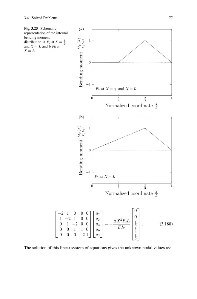
Fig. 3.25 Schematic
representation of the internal
bending moment
distribution: a F 0 at X =
L
3
and X = L and b F 0 at
X = L
(a)
0
1
3
2
3
1
−1
0
1
F0 at X =
L
3
and X = L
Normalized coordinate
X
L
Bending moment
M
Y (X)
F
0 L/3
(b)
0
1
3
2
3
1
−1
0
1
F0 at X = L
Normalized coordinate
X
L
Bending moment
M
Y (X)
F
0 L/3
⎡
⎢
⎢
⎢
⎢
⎣
−2 1 0 0 0
1 −2 1 0 0
0 1 −2 0 0
0 0 1 1 0
0 0 0 −2 1
⎤
⎥
⎥
⎥
⎥
⎦
⎡
⎢
⎢
⎢
⎢
⎣
u 2
u 3
u 4
u 6
u 7
⎤
⎥
⎥
⎥
⎥
⎦
= −
X
2 F 0 L
E I Y
⎡
⎢
⎢
⎢
⎢
⎢
⎢
⎣
0
0
1
6
1
3
1
6
⎤
⎥
⎥
⎥
⎥
⎥
⎥
⎦
.
(3.188)
The solution of this linear system of equations gives the unknown nodal values as:
77
Fig. 3.25 Schematic
representation of the internal
bending moment
distribution: a F 0 at X =
L
3
and X = L and b F 0 at
X = L
(a)
0
1
3
2
3
1
−1
0
1
F0 at X =
L
3
and X = L
Normalized coordinate
X
L
Bending moment
M
Y (X)
F
0 L/3
(b)
0
1
3
2
3
1
−1
0
1
F0 at X = L
Normalized coordinate
X
L
Bending moment
M
Y (X)
F
0 L/3
⎡
⎢
⎢
⎢
⎢
⎣
−2 1 0 0 0
1 −2 1 0 0
0 1 −2 0 0
0 0 1 1 0
0 0 0 −2 1
⎤
⎥
⎥
⎥
⎥
⎦
⎡
⎢
⎢
⎢
⎢
⎣
u 2
u 3
u 4
u 6
u 7
⎤
⎥
⎥
⎥
⎥
⎦
= −
X
2 F 0 L
E I Y
⎡
⎢
⎢
⎢
⎢
⎢
⎢
⎣
0
0
1
6
1
3
1
6
⎤
⎥
⎥
⎥
⎥
⎥
⎥
⎦
.
(3.188)
The solution of this linear system of equations gives the unknown nodal values as: