

50
3 Investigation of Euler–Bernoulli Beams in the Elastic Range
node 5:
E I Y
X 3 (u 7 − 4u 6 + 6u 5 − 4u 4 + u 3 ) = −F 0 .
(3.47)
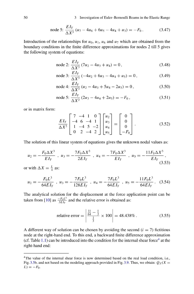
Introduction of the relationships for u 0 , u 1 , u 6 and u 7 which are obtained from the
boundary conditions in the finite difference approximations for nodes 2 till 5 gives
the following system of equations:
node 2:
E I Y
X 3 (7u 2 − 4u 3 + u 4 ) = 0 ,
(3.48)
node 3:
E I Y
X 3 (−4u 2 + 6u 3 − 4u 4 + u 5 ) = 0 ,
(3.49)
node 4:
E I Y
X 3 (u 2 − 4u 3 + 5u 4 − 2u 5 ) = 0 ,
(3.50)
node 5:
E I Y
X 3 (2u 3 − 4u 4 + 2u 5 ) = −F 0 ,
(3.51)
or in matrix form:
E I Y
X 3
⎡
⎢
⎢
⎣
7 −4 1 0
−4 6 −4 1
1 −4 5 −2
0 2 −4 2
⎤
⎥
⎥
⎦
⎡
⎢
⎢
⎣
u 2
u 3
u 4
u 5
⎤
⎥
⎥
⎦ =
⎡
⎢
⎢
⎣
0
0
0
−F 0
⎤
⎥
⎥
⎦ .
(3.52)
The solution of this linear system of equations gives the unknown nodal values as:
u 2 = −
F 0 X
3
E I Y
, u 3 = −
7F 0 X
3
2E I Y
, u 4 = −
7F 0 X
3
E I Y
, u 5 = −
11F 0 X
3
E I Y
,
(3.53)
or with X =
L
4
as:
u 2 = −
F 0 L
3
64E I Y
, u 3 = −
7F 0 L
3
128E I Y
, u 4 = −
7F 0 L
3
64E I Y
, u 5 = −
11F 0 L
3
64E I Y
. (3.54)
The analytical solution for the displacement at the force application point can be
taken from [10] as
−F 0 L
3
3E I Y
and the relative error is obtained as:
relative error =
11
64
−
1
3
1
3
× 100
= 48.438% .
(3.55)
A different way of solution can be chosen by avoiding the second (i = 7) fictitious
node at the right-hand end. To this end, a backward finite difference approximation
(cf. Table 1.1) can be introduced into the condition for the internal shear force
4 at the
right-hand end:
4 The value of the internal shear force is now determined based on the real load condition, i.e.,
Fig. 3.5b, and not based on the modeling approach provided in Fig. 3.9. Thus, we obtain: Q Z (X =
L) = −F 0 .
3 Investigation of Euler–Bernoulli Beams in the Elastic Range
node 5:
E I Y
X 3 (u 7 − 4u 6 + 6u 5 − 4u 4 + u 3 ) = −F 0 .
(3.47)
Introduction of the relationships for u 0 , u 1 , u 6 and u 7 which are obtained from the
boundary conditions in the finite difference approximations for nodes 2 till 5 gives
the following system of equations:
node 2:
E I Y
X 3 (7u 2 − 4u 3 + u 4 ) = 0 ,
(3.48)
node 3:
E I Y
X 3 (−4u 2 + 6u 3 − 4u 4 + u 5 ) = 0 ,
(3.49)
node 4:
E I Y
X 3 (u 2 − 4u 3 + 5u 4 − 2u 5 ) = 0 ,
(3.50)
node 5:
E I Y
X 3 (2u 3 − 4u 4 + 2u 5 ) = −F 0 ,
(3.51)
or in matrix form:
E I Y
X 3
⎡
⎢
⎢
⎣
7 −4 1 0
−4 6 −4 1
1 −4 5 −2
0 2 −4 2
⎤
⎥
⎥
⎦
⎡
⎢
⎢
⎣
u 2
u 3
u 4
u 5
⎤
⎥
⎥
⎦ =
⎡
⎢
⎢
⎣
0
0
0
−F 0
⎤
⎥
⎥
⎦ .
(3.52)
The solution of this linear system of equations gives the unknown nodal values as:
u 2 = −
F 0 X
3
E I Y
, u 3 = −
7F 0 X
3
2E I Y
, u 4 = −
7F 0 X
3
E I Y
, u 5 = −
11F 0 X
3
E I Y
,
(3.53)
or with X =
L
4
as:
u 2 = −
F 0 L
3
64E I Y
, u 3 = −
7F 0 L
3
128E I Y
, u 4 = −
7F 0 L
3
64E I Y
, u 5 = −
11F 0 L
3
64E I Y
. (3.54)
The analytical solution for the displacement at the force application point can be
taken from [10] as
−F 0 L
3
3E I Y
and the relative error is obtained as:
relative error =
11
64
−
1
3
1
3
× 100
= 48.438% .
(3.55)
A different way of solution can be chosen by avoiding the second (i = 7) fictitious
node at the right-hand end. To this end, a backward finite difference approximation
(cf. Table 1.1) can be introduced into the condition for the internal shear force
4 at the
right-hand end:
4 The value of the internal shear force is now determined based on the real load condition, i.e.,
Fig. 3.5b, and not based on the modeling approach provided in Fig. 3.9. Thus, we obtain: Q Z (X =
L) = −F 0 .