

3.4 Solved Problems
51
E I Y
5u 5 − 18u 4 + 24u 3 − 14u 2 + 3u 1
2X 3
d 3 u
dX 3
5
= −Q Z (X = L) = F 0 .
(3.56)
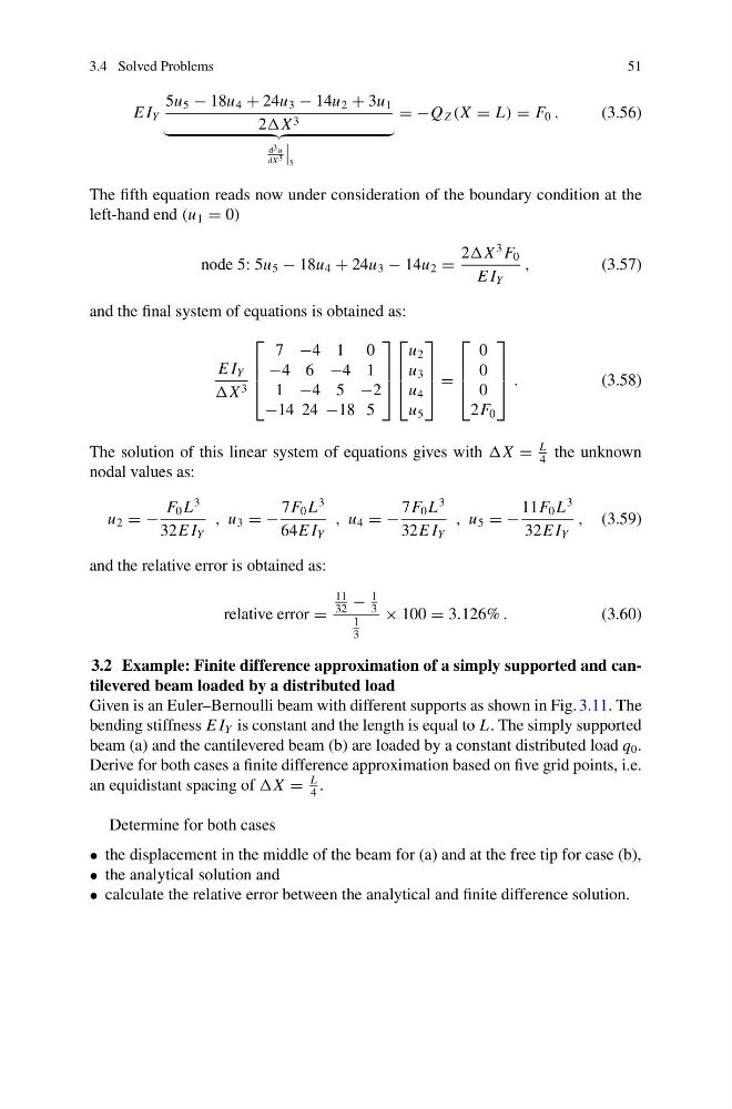
The fifth equation reads now under consideration of the boundary condition at the
left-hand end (u 1 = 0)
node 5: 5u 5 − 18u 4 + 24u 3 − 14u 2 =
2X
3 F 0
E I Y
,
(3.57)
and the final system of equations is obtained as:
E I Y
X 3
⎡
⎢
⎢
⎣
7 −4 1 0
−4 6 −4 1
1 −4 5 −2
−14 24 −18 5
⎤
⎥
⎥
⎦
⎡
⎢
⎢
⎣
u 2
u 3
u 4
u 5
⎤
⎥
⎥
⎦ =
⎡
⎢
⎢
⎣
0
0
0
2F 0
⎤
⎥
⎥
⎦ .
(3.58)
The solution of this linear system of equations gives with X =
L
4
the unknown
nodal values as:
u 2 = −
F 0 L
3
32E I Y
, u 3 = −
7F 0 L
3
64E I Y
, u 4 = −
7F 0 L
3
32E I Y
, u 5 = −
11F 0 L
3
32E I Y
, (3.59)
and the relative error is obtained as:
relative error =
11
32
−
1
3
1
3
× 100 = 3.126% .
(3.60)
3.2 Example: Finite difference approximation of a simply supported and cantilevered beam loaded by a distributed load
Given is an Euler–Bernoulli beam with different supports as shown in Fig. 3.11. The
bending stiffness E I Y is constant and the length is equal to L. The simply supported
beam (a) and the cantilevered beam (b) are loaded by a constant distributed load q 0 .
Derive for both cases a finite difference approximation based on five grid points, i.e.
an equidistant spacing of X =
L
4
.
Determine for both cases
• the displacement in the middle of the beam for (a) and at the free tip for case (b),
• the analytical solution and
• calculate the relative error between the analytical and finite difference solution.
51
E I Y
5u 5 − 18u 4 + 24u 3 − 14u 2 + 3u 1
2X 3
d 3 u
dX 3
5
= −Q Z (X = L) = F 0 .
(3.56)
The fifth equation reads now under consideration of the boundary condition at the
left-hand end (u 1 = 0)
node 5: 5u 5 − 18u 4 + 24u 3 − 14u 2 =
2X
3 F 0
E I Y
,
(3.57)
and the final system of equations is obtained as:
E I Y
X 3
⎡
⎢
⎢
⎣
7 −4 1 0
−4 6 −4 1
1 −4 5 −2
−14 24 −18 5
⎤
⎥
⎥
⎦
⎡
⎢
⎢
⎣
u 2
u 3
u 4
u 5
⎤
⎥
⎥
⎦ =
⎡
⎢
⎢
⎣
0
0
0
2F 0
⎤
⎥
⎥
⎦ .
(3.58)
The solution of this linear system of equations gives with X =
L
4
the unknown
nodal values as:
u 2 = −
F 0 L
3
32E I Y
, u 3 = −
7F 0 L
3
64E I Y
, u 4 = −
7F 0 L
3
32E I Y
, u 5 = −
11F 0 L
3
32E I Y
, (3.59)
and the relative error is obtained as:
relative error =
11
32
−
1
3
1
3
× 100 = 3.126% .
(3.60)
3.2 Example: Finite difference approximation of a simply supported and cantilevered beam loaded by a distributed load
Given is an Euler–Bernoulli beam with different supports as shown in Fig. 3.11. The
bending stiffness E I Y is constant and the length is equal to L. The simply supported
beam (a) and the cantilevered beam (b) are loaded by a constant distributed load q 0 .
Derive for both cases a finite difference approximation based on five grid points, i.e.
an equidistant spacing of X =
L
4
.
Determine for both cases
• the displacement in the middle of the beam for (a) and at the free tip for case (b),
• the analytical solution and
• calculate the relative error between the analytical and finite difference solution.