

2.4 Solved Problems
33
node 5: E
0 +
A
X 2 × (u 6 − 2u 5 + u 4 )
= 0 .
(2.101)
Replacing in Eq. (2.101) the fictitious node again by Eq. (2.90), i.e.,
u 6 = u 4 +
2X F 0
E 5 A 5
,
(2.102)
the following system of equations can be stated:
⎡
⎢
⎢
⎣
−2 1 0 0
7 −12 5 0
0 1 −2 1
0 0 2 −2
⎤
⎥
⎥
⎦
⎡
⎢
⎢
⎣
u 2
u 3
u 4
u 5
⎤
⎥
⎥
⎦ =
X F 0
E A
⎡
⎢
⎢
⎣
0
0
0
−2
⎤
⎥
⎥
⎦ .
(2.103)
The solution of this linear system of equations gives the unknown nodal values as:
⎡
⎢
⎢
⎣
u 2
u 3
u 4
u 5
⎤
⎥
⎥
⎦ =
F 0 L
E A
⎡
⎢
⎢
⎢
⎣
5
28
5
14
17
28
6
7
⎤
⎥
⎥
⎥
⎦
=
F 0 L
E A
⎡
⎢
⎢
⎢
⎣
0.17857143
0.35714286
0.60714286
0.85714286
⎤
⎥
⎥
⎥
⎦
.
(2.104)
2.5 Supplementary Problems
2.3 Finite difference approximation of a cantilevered rod with distributed load
based on five domain nodes
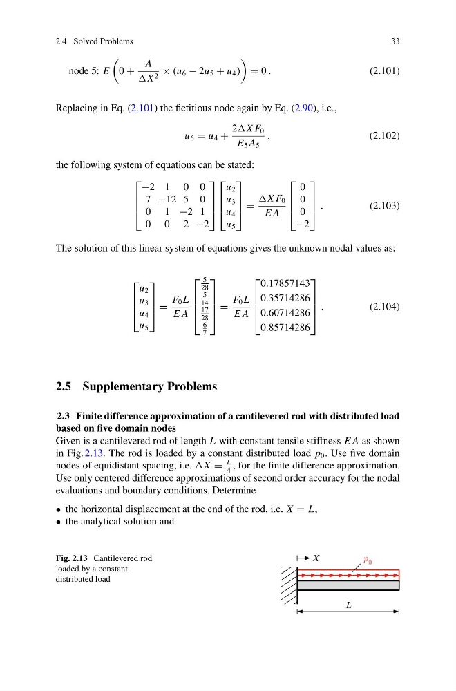
Given is a cantilevered rod of length L with constant tensile stiffness E A as shown
in Fig. 2.13. The rod is loaded by a constant distributed load p 0 . Use five domain
nodes of equidistant spacing, i.e. =
L
4
, for the finite difference approximation.
Use only centered difference approximations of second order accuracy for the nodal
evaluations and boundary conditions. Determine
• the horizontal displacement at the end of the rod, i.e. X = L,
• the analytical solution and
Fig. 2.13 Cantilevered rod
loaded by a constant
distributed load
33
node 5: E
0 +
A
X 2 × (u 6 − 2u 5 + u 4 )
= 0 .
(2.101)
Replacing in Eq. (2.101) the fictitious node again by Eq. (2.90), i.e.,
u 6 = u 4 +
2X F 0
E 5 A 5
,
(2.102)
the following system of equations can be stated:
⎡
⎢
⎢
⎣
−2 1 0 0
7 −12 5 0
0 1 −2 1
0 0 2 −2
⎤
⎥
⎥
⎦
⎡
⎢
⎢
⎣
u 2
u 3
u 4
u 5
⎤
⎥
⎥
⎦ =
X F 0
E A
⎡
⎢
⎢
⎣
0
0
0
−2
⎤
⎥
⎥
⎦ .
(2.103)
The solution of this linear system of equations gives the unknown nodal values as:
⎡
⎢
⎢
⎣
u 2
u 3
u 4
u 5
⎤
⎥
⎥
⎦ =
F 0 L
E A
⎡
⎢
⎢
⎢
⎣
5
28
5
14
17
28
6
7
⎤
⎥
⎥
⎥
⎦
=
F 0 L
E A
⎡
⎢
⎢
⎢
⎣
0.17857143
0.35714286
0.60714286
0.85714286
⎤
⎥
⎥
⎥
⎦
.
(2.104)
2.5 Supplementary Problems
2.3 Finite difference approximation of a cantilevered rod with distributed load
based on five domain nodes
Given is a cantilevered rod of length L with constant tensile stiffness E A as shown
in Fig. 2.13. The rod is loaded by a constant distributed load p 0 . Use five domain
nodes of equidistant spacing, i.e. =
L
4
, for the finite difference approximation.
Use only centered difference approximations of second order accuracy for the nodal
evaluations and boundary conditions. Determine
• the horizontal displacement at the end of the rod, i.e. X = L,
• the analytical solution and
Fig. 2.13 Cantilevered rod
loaded by a constant
distributed load