

32
2 Investigation of Rods in the Elastic Range
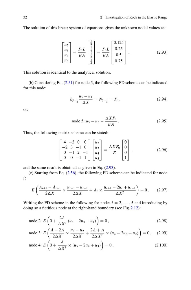
The solution of this linear system of equations gives the unknown nodal values as:
⎡
⎢
⎢
⎣
u 2
u 3
u 4
u 5
⎤
⎥
⎥
⎦ =
F 0 L
E A
⎡
⎢
⎢
⎢
⎣
1
8
1
4
1
2
3
4
⎤
⎥
⎥
⎥
⎦
=
F 0 L
E A
⎡
⎢
⎢
⎢
⎣
0.125
0.25
0.5
0.75
⎤
⎥
⎥
⎥
⎦
.
(2.93)
This solution is identical to the analytical solution.
(b) Considering Eq. (2.51) for node 5, the following FD scheme can be indicated
for this node:
k 5−
1
2
u 5 − u 4
X
= N 5−
1
2
= F 0 ,
(2.94)
or:
node 5: u 5 − u 5 −
X F 0
E A
.
(2.95)
Thus, the following matrix scheme can be stated:
⎡
⎢
⎢
⎣
4 −2 0 0
−2 3 −1 0
0 −1 2 −1
0 0 −1 1
⎤
⎥
⎥
⎦
⎡
⎢
⎢
⎣
u 2
u 3
u 4
u 5
⎤
⎥
⎥
⎦ =
X F 0
E
⎡
⎢
⎢
⎣
0
0
0
1
⎤
⎥
⎥
⎦ ,
(2.96)
and the same result is obtained as given in Eq. (2.93).
(c) Starting from Eq. (2.56), the following FD scheme can be indicated for node
i:
E
A i+1 − A i−1
2X
×
u i+1 − u i−1
2X
+ A i ×
u i+1 − 2u i + u i−1
X 2
= 0 .
(2.97)
Writing the FD scheme in the following for nodes i = 2, . . . , 5 and introducing by
doing so a fictitious node at the right-hand boundary (see Fig. 2.12):
node 2: E
0 +
2 A
X 2 (u 3 − 2u 2 + u 1 )
= 0 ,
(2.98)
node 3: E
A − 2 A
2X
×
u 4 − u 2
2X
+
2 A + A
2X 2 × (u 4 − 2u 3 + u 2 )
= 0 , (2.99)
node 4: E
0 +
A
X 2 × (u 5 − 2u 4 + u 3 )
= 0 ,
(2.100)
2 Investigation of Rods in the Elastic Range
The solution of this linear system of equations gives the unknown nodal values as:
⎡
⎢
⎢
⎣
u 2
u 3
u 4
u 5
⎤
⎥
⎥
⎦ =
F 0 L
E A
⎡
⎢
⎢
⎢
⎣
1
8
1
4
1
2
3
4
⎤
⎥
⎥
⎥
⎦
=
F 0 L
E A
⎡
⎢
⎢
⎢
⎣
0.125
0.25
0.5
0.75
⎤
⎥
⎥
⎥
⎦
.
(2.93)
This solution is identical to the analytical solution.
(b) Considering Eq. (2.51) for node 5, the following FD scheme can be indicated
for this node:
k 5−
1
2
u 5 − u 4
X
= N 5−
1
2
= F 0 ,
(2.94)
or:
node 5: u 5 − u 5 −
X F 0
E A
.
(2.95)
Thus, the following matrix scheme can be stated:
⎡
⎢
⎢
⎣
4 −2 0 0
−2 3 −1 0
0 −1 2 −1
0 0 −1 1
⎤
⎥
⎥
⎦
⎡
⎢
⎢
⎣
u 2
u 3
u 4
u 5
⎤
⎥
⎥
⎦ =
X F 0
E
⎡
⎢
⎢
⎣
0
0
0
1
⎤
⎥
⎥
⎦ ,
(2.96)
and the same result is obtained as given in Eq. (2.93).
(c) Starting from Eq. (2.56), the following FD scheme can be indicated for node
i:
E
A i+1 − A i−1
2X
×
u i+1 − u i−1
2X
+ A i ×
u i+1 − 2u i + u i−1
X 2
= 0 .
(2.97)
Writing the FD scheme in the following for nodes i = 2, . . . , 5 and introducing by
doing so a fictitious node at the right-hand boundary (see Fig. 2.12):
node 2: E
0 +
2 A
X 2 (u 3 − 2u 2 + u 1 )
= 0 ,
(2.98)
node 3: E
A − 2 A
2X
×
u 4 − u 2
2X
+
2 A + A
2X 2 × (u 4 − 2u 3 + u 2 )
= 0 , (2.99)
node 4: E
0 +
A
X 2 × (u 5 − 2u 4 + u 3 )
= 0 ,
(2.100)