

28
2 Investigation of Rods in the Elastic Range
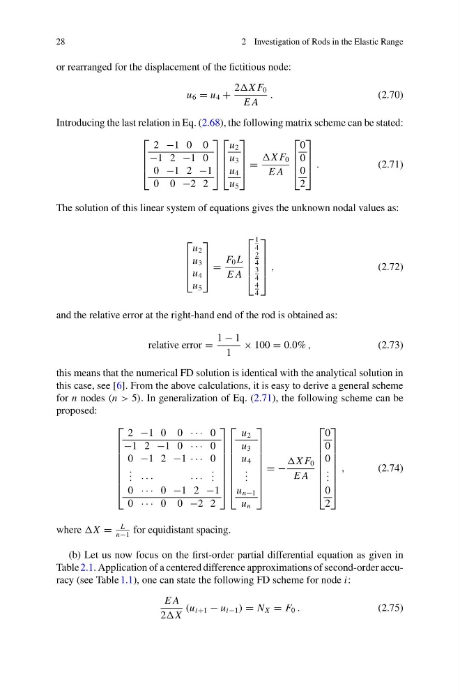
or rearranged for the displacement of the fictitious node:
u 6 = u 4 +
2X F 0
E A
.
(2.70)
Introducing the last relation in Eq. (2.68), the following matrix scheme can be stated:
⎡
⎢
⎢
⎣
2 −1 0 0
−1 2 −1 0
0 −1 2 −1
0 0 −2 2
⎤
⎥
⎥
⎦
⎡
⎢
⎢
⎣
u 2
u 3
u 4
u 5
⎤
⎥
⎥
⎦ =
X F 0
E A
⎡
⎢
⎢
⎣
0
0
0
2
⎤
⎥
⎥
⎦ .
(2.71)
The solution of this linear system of equations gives the unknown nodal values as:
⎡
⎢
⎢
⎣
u 2
u 3
u 4
u 5
⎤
⎥
⎥
⎦ =
F 0 L
E A
⎡
⎢
⎢
⎢
⎣
1
4
2
4
3
4
4
4
⎤
⎥
⎥
⎥
⎦
,
(2.72)
and the relative error at the right-hand end of the rod is obtained as:
relative error =
1 − 1
1
× 100 = 0.0% ,
(2.73)
this means that the numerical FD solution is identical with the analytical solution in
this case, see [6]. From the above calculations, it is easy to derive a general scheme
for n nodes (n > 5). In generalization of Eq. (2.71), the following scheme can be
proposed:
⎡
⎢
⎢
⎢
⎢
⎢
⎢
⎢
⎣
2 −1 0 0 · · · 0
−1 2 −1 0 · · · 0
0 −1 2 −1 · · · 0
. . . · · ·
· · ·
. . .
0 · · · 0 −1 2 −1
0 · · · 0 0 −2 2
⎤
⎥
⎥
⎥
⎥
⎥
⎥
⎥
⎦
⎡
⎢
⎢
⎢
⎢
⎢
⎢
⎢
⎣
u 2
u 3
u 4
. . .
u n−1
u n
⎤
⎥
⎥
⎥
⎥
⎥
⎥
⎥
⎦
= −
X F 0
E A
⎡
⎢
⎢
⎢
⎢
⎢
⎢
⎢
⎣
0
0
0
. . .
0
2
⎤
⎥
⎥
⎥
⎥
⎥
⎥
⎥
⎦
,
(2.74)
where X =
L
n−1
for equidistant spacing.
(b) Let us now focus on the first-order partial differential equation as given in
Table 2.1. Application of a centered difference approximations of second-order accuracy (see Table 1.1), one can state the following FD scheme for node i:
E A
2X
(u i+1 − u i−1 ) = N X = F 0 .
(2.75)
2 Investigation of Rods in the Elastic Range
or rearranged for the displacement of the fictitious node:
u 6 = u 4 +
2X F 0
E A
.
(2.70)
Introducing the last relation in Eq. (2.68), the following matrix scheme can be stated:
⎡
⎢
⎢
⎣
2 −1 0 0
−1 2 −1 0
0 −1 2 −1
0 0 −2 2
⎤
⎥
⎥
⎦
⎡
⎢
⎢
⎣
u 2
u 3
u 4
u 5
⎤
⎥
⎥
⎦ =
X F 0
E A
⎡
⎢
⎢
⎣
0
0
0
2
⎤
⎥
⎥
⎦ .
(2.71)
The solution of this linear system of equations gives the unknown nodal values as:
⎡
⎢
⎢
⎣
u 2
u 3
u 4
u 5
⎤
⎥
⎥
⎦ =
F 0 L
E A
⎡
⎢
⎢
⎢
⎣
1
4
2
4
3
4
4
4
⎤
⎥
⎥
⎥
⎦
,
(2.72)
and the relative error at the right-hand end of the rod is obtained as:
relative error =
1 − 1
1
× 100 = 0.0% ,
(2.73)
this means that the numerical FD solution is identical with the analytical solution in
this case, see [6]. From the above calculations, it is easy to derive a general scheme
for n nodes (n > 5). In generalization of Eq. (2.71), the following scheme can be
proposed:
⎡
⎢
⎢
⎢
⎢
⎢
⎢
⎢
⎣
2 −1 0 0 · · · 0
−1 2 −1 0 · · · 0
0 −1 2 −1 · · · 0
. . . · · ·
· · ·
. . .
0 · · · 0 −1 2 −1
0 · · · 0 0 −2 2
⎤
⎥
⎥
⎥
⎥
⎥
⎥
⎥
⎦
⎡
⎢
⎢
⎢
⎢
⎢
⎢
⎢
⎣
u 2
u 3
u 4
. . .
u n−1
u n
⎤
⎥
⎥
⎥
⎥
⎥
⎥
⎥
⎦
= −
X F 0
E A
⎡
⎢
⎢
⎢
⎢
⎢
⎢
⎢
⎣
0
0
0
. . .
0
2
⎤
⎥
⎥
⎥
⎥
⎥
⎥
⎥
⎦
,
(2.74)
where X =
L
n−1
for equidistant spacing.
(b) Let us now focus on the first-order partial differential equation as given in
Table 2.1. Application of a centered difference approximations of second-order accuracy (see Table 1.1), one can state the following FD scheme for node i:
E A
2X
(u i+1 − u i−1 ) = N X = F 0 .
(2.75)