

2.3 Varying Material and Geometry Parameters
25
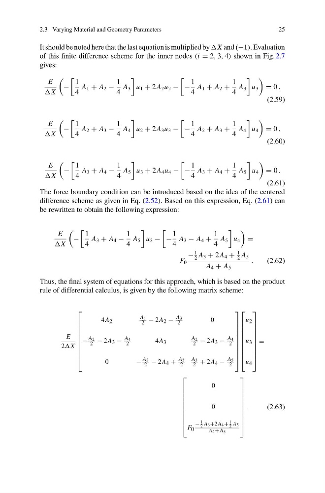
It should be noted here that the last equation is multiplied by X and (−1). Evaluation
of this finite difference scheme for the inner nodes (i = 2, 3, 4) shown in Fig. 2.7
gives:
E
X
−
1
4
A 1 + A 2 −
1
4
A 3
u 1 + 2 A 2 u 2 −
−
1
4
A 1 + A 2 +
1
4
A 3
u 3
= 0 ,
(2.59)
E
X
−
1
4
A 2 + A 3 −
1
4
A 4
u 2 + 2 A 3 u 3 −
−
1
4
A 2 + A 3 +
1
4
A 4
u 4
= 0 ,
(2.60)
E
X
−
1
4
A 3 + A 4 −
1
4
A 5
u 3 + 2 A 4 u 4 −
−
1
4
A 3 + A 4 +
1
4
A 5
u 4
= 0 .
(2.61)
The force boundary condition can be introduced based on the idea of the centered
difference scheme as given in Eq. (2.52). Based on this expression, Eq. (2.61) can
be rewritten to obtain the following expression:
E
X
−
1
4
A 3 + A 4 −
1
4
A 5
u 3 −
−
1
4
A 3 − A 4 +
1
4
A 5
u 4
=
F 0
−
1
2
A 3 + 2 A 4 +
1
2
A 5
A 4 + A 5
.
(2.62)
Thus, the final system of equations for this approach, which is based on the product
rule of differential calculus, is given by the following matrix scheme:
E
2X
⎡
⎢
⎢
⎢
⎢
⎢
⎢
⎢
⎢
⎢
⎣
4 A 2
A 1
2 − 2 A 2 −
A 3
2
0
−
A 2
2 − 2 A 3 −
A 4
2
4 A 3
A 2
2 − 2 A 3 −
A 4
2
0
−
A 3
2 − 2 A 4 +
A 5
2
A 3
2 + 2 A 4 −
A 5
2
⎤
⎥
⎥
⎥
⎥
⎥
⎥
⎥
⎥
⎥
⎦
⎡
⎢
⎢
⎢
⎢
⎢
⎢
⎢
⎢
⎢
⎣
u 2
u 3
u 4
⎤
⎥
⎥
⎥
⎥
⎥
⎥
⎥
⎥
⎥
⎦
=
⎡
⎢
⎢
⎢
⎢
⎢
⎢
⎢
⎢
⎢
⎣
0
0
F 0
−
1
2 A 3 +2 A 4 +
1
2 A 5
A 4 +A 5
⎤
⎥
⎥
⎥
⎥
⎥
⎥
⎥
⎥
⎥
⎦
.
(2.63)
25
It should be noted here that the last equation is multiplied by X and (−1). Evaluation
of this finite difference scheme for the inner nodes (i = 2, 3, 4) shown in Fig. 2.7
gives:
E
X
−
1
4
A 1 + A 2 −
1
4
A 3
u 1 + 2 A 2 u 2 −
−
1
4
A 1 + A 2 +
1
4
A 3
u 3
= 0 ,
(2.59)
E
X
−
1
4
A 2 + A 3 −
1
4
A 4
u 2 + 2 A 3 u 3 −
−
1
4
A 2 + A 3 +
1
4
A 4
u 4
= 0 ,
(2.60)
E
X
−
1
4
A 3 + A 4 −
1
4
A 5
u 3 + 2 A 4 u 4 −
−
1
4
A 3 + A 4 +
1
4
A 5
u 4
= 0 .
(2.61)
The force boundary condition can be introduced based on the idea of the centered
difference scheme as given in Eq. (2.52). Based on this expression, Eq. (2.61) can
be rewritten to obtain the following expression:
E
X
−
1
4
A 3 + A 4 −
1
4
A 5
u 3 −
−
1
4
A 3 − A 4 +
1
4
A 5
u 4
=
F 0
−
1
2
A 3 + 2 A 4 +
1
2
A 5
A 4 + A 5
.
(2.62)
Thus, the final system of equations for this approach, which is based on the product
rule of differential calculus, is given by the following matrix scheme:
E
2X
⎡
⎢
⎢
⎢
⎢
⎢
⎢
⎢
⎢
⎢
⎣
4 A 2
A 1
2 − 2 A 2 −
A 3
2
0
−
A 2
2 − 2 A 3 −
A 4
2
4 A 3
A 2
2 − 2 A 3 −
A 4
2
0
−
A 3
2 − 2 A 4 +
A 5
2
A 3
2 + 2 A 4 −
A 5
2
⎤
⎥
⎥
⎥
⎥
⎥
⎥
⎥
⎥
⎥
⎦
⎡
⎢
⎢
⎢
⎢
⎢
⎢
⎢
⎢
⎢
⎣
u 2
u 3
u 4
⎤
⎥
⎥
⎥
⎥
⎥
⎥
⎥
⎥
⎥
⎦
=
⎡
⎢
⎢
⎢
⎢
⎢
⎢
⎢
⎢
⎢
⎣
0
0
F 0
−
1
2 A 3 +2 A 4 +
1
2 A 5
A 4 +A 5
⎤
⎥
⎥
⎥
⎥
⎥
⎥
⎥
⎥
⎥
⎦
.
(2.63)