

24
2 Investigation of Rods in the Elastic Range
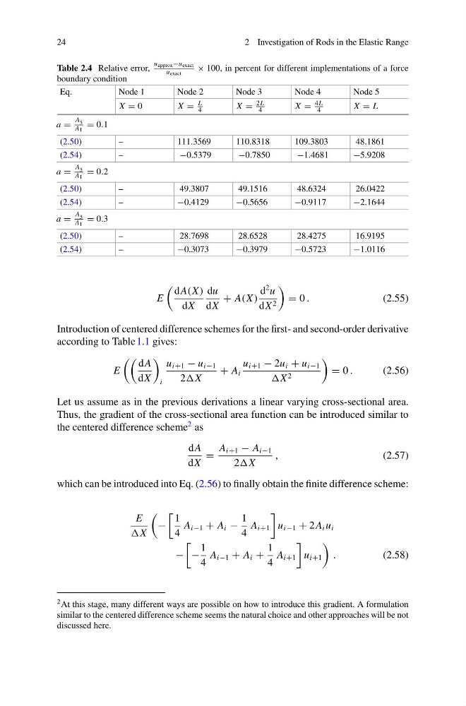
Table 2.4 Relative error,
uapprox−uexact
uexact
× 100, in percent for different implementations of a force
boundary condition
Eq.
Node 1
Node 2
Node 3
Node 4
Node 5
X = 0
X =
L
4
X =
2L
4
X =
4L
4
X = L
a =
A 5
A1 = 0.1
(2.50)
–
111.3569
110.8318
109.3803
48.1861
(2.54)
–
−0.5379
−0.7850
−1.4681
−5.9208
a =
A 5
A1 = 0.2
(2.50)
–
49.3807
49.1516
48.6324
26.0422
(2.54)
–
−0.4129
−0.5656
−0.9117
−2.1644
a =
A 5
A1 = 0.3
(2.50)
–
28.7698
28.6528
28.4275
16.9195
(2.54)
–
−0.3073
−0.3979
−0.5723
−1.0116
E
dA(X )
dX
du
dX
+ A(X )
d
2 u
dX 2
= 0 .
(2.55)
Introduction of centered difference schemes for the first- and second-order derivative
according to Table 1.1 gives:
E
dA
dX
i
u i+1 − u i−1
2X
+ A i
u i+1 − 2u i + u i−1
X 2
= 0 .
(2.56)
Let us assume as in the previous derivations a linear varying cross-sectional area.
Thus, the gradient of the cross-sectional area function can be introduced similar to
the centered difference scheme
2 as
dA
dX
=
A i+1 − A i−1
2X
,
(2.57)
which can be introduced into Eq. (2.56) to finally obtain the finite difference scheme:
E
X
−
1
4
A i−1 + A i −
1
4
A i+1
u i−1 + 2 A i u i
−
−
1
4
A i−1 + A i +
1
4
A i+1
u i+1
.
(2.58)
2 At this stage, many different ways are possible on how to introduce this gradient. A formulation
similar to the centered difference scheme seems the natural choice and other approaches will be not
discussed here.
2 Investigation of Rods in the Elastic Range
Table 2.4 Relative error,
uapprox−uexact
uexact
× 100, in percent for different implementations of a force
boundary condition
Eq.
Node 1
Node 2
Node 3
Node 4
Node 5
X = 0
X =
L
4
X =
2L
4
X =
4L
4
X = L
a =
A 5
A1 = 0.1
(2.50)
–
111.3569
110.8318
109.3803
48.1861
(2.54)
–
−0.5379
−0.7850
−1.4681
−5.9208
a =
A 5
A1 = 0.2
(2.50)
–
49.3807
49.1516
48.6324
26.0422
(2.54)
–
−0.4129
−0.5656
−0.9117
−2.1644
a =
A 5
A1 = 0.3
(2.50)
–
28.7698
28.6528
28.4275
16.9195
(2.54)
–
−0.3073
−0.3979
−0.5723
−1.0116
E
dA(X )
dX
du
dX
+ A(X )
d
2 u
dX 2
= 0 .
(2.55)
Introduction of centered difference schemes for the first- and second-order derivative
according to Table 1.1 gives:
E
dA
dX
i
u i+1 − u i−1
2X
+ A i
u i+1 − 2u i + u i−1
X 2
= 0 .
(2.56)
Let us assume as in the previous derivations a linear varying cross-sectional area.
Thus, the gradient of the cross-sectional area function can be introduced similar to
the centered difference scheme
2 as
dA
dX
=
A i+1 − A i−1
2X
,
(2.57)
which can be introduced into Eq. (2.56) to finally obtain the finite difference scheme:
E
X
−
1
4
A i−1 + A i −
1
4
A i+1
u i−1 + 2 A i u i
−
−
1
4
A i−1 + A i +
1
4
A i+1
u i+1
.
(2.58)
2 At this stage, many different ways are possible on how to introduce this gradient. A formulation
similar to the centered difference scheme seems the natural choice and other approaches will be not
discussed here.