

2.3 Varying Material and Geometry Parameters
23
du
dX
i−
1
2
=
u i − u i−1
X
=
N i−
1
2
k i−
1
2
,
(2.51)
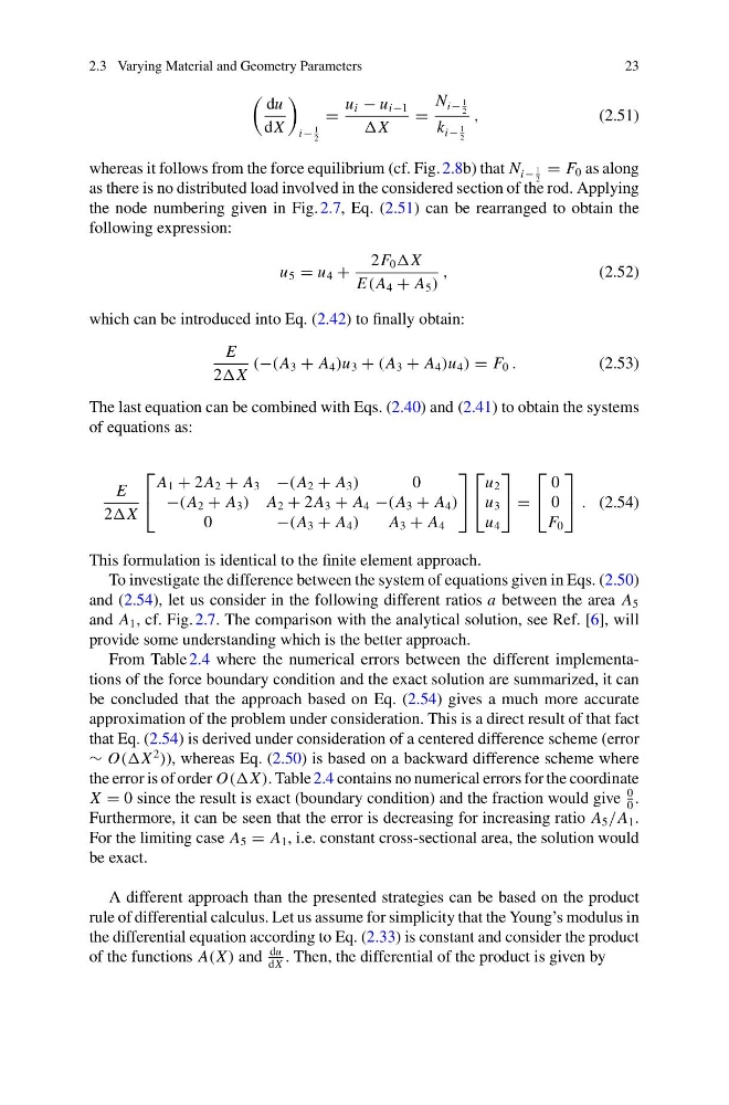
whereas it follows from the force equilibrium (cf. Fig. 2.8b) that N i−
1
2
= F 0 as along
as there is no distributed load involved in the considered section of the rod. Applying
the node numbering given in Fig. 2.7, Eq. (2.51) can be rearranged to obtain the
following expression:
u 5 = u 4 +
2F 0 X
E(A 4 + A 5 )
,
(2.52)
which can be introduced into Eq. (2.42) to finally obtain:
E
2X
(−(A 3 + A 4 )u 3 + (A 3 + A 4 )u 4 ) = F 0 .
(2.53)
The last equation can be combined with Eqs. (2.40) and (2.41) to obtain the systems
of equations as:
E
2X
⎡
⎣
A 1 + 2 A 2 + A 3 −(A 2 + A 3 )
0
−(A 2 + A 3 ) A 2 + 2 A 3 + A 4 −(A 3 + A 4 )
0
−(A 3 + A 4 )
A 3 + A 4
⎤
⎦
⎡
⎣
u 2
u 3
u 4
⎤
⎦ =
⎡
⎣
0
0
F 0
⎤
⎦ . (2.54)
This formulation is identical to the finite element approach.
To investigate the difference between the system of equations given in Eqs. (2.50)
and (2.54), let us consider in the following different ratios a between the area A 5
and A 1 , cf. Fig. 2.7. The comparison with the analytical solution, see Ref. [6], will
provide some understanding which is the better approach.
From Table 2.4 where the numerical errors between the different implementations of the force boundary condition and the exact solution are summarized, it can
be concluded that the approach based on Eq. (2.54) gives a much more accurate
approximation of the problem under consideration. This is a direct result of that fact
that Eq. (2.54) is derived under consideration of a centered difference scheme (error
∼ O((X
2
)), whereas Eq. (2.50) is based on a backward difference scheme where
the error is of order O((X ). Table 2.4 contains no numerical errors for the coordinate
X = 0 since the result is exact (boundary condition) and the fraction would give
0
0
.
Furthermore, it can be seen that the error is decreasing for increasing ratio A 5 /A 1 .
For the limiting case A 5 = A 1 , i.e. constant cross-sectional area, the solution would
be exact.
A different approach than the presented strategies can be based on the product
rule of differential calculus. Let us assume for simplicity that the Young’s modulus in
the differential equation according to Eq. (2.33) is constant and consider the product
of the functions A(X ) and
du
dX
. Then, the differential of the product is given by
23
du
dX
i−
1
2
=
u i − u i−1
X
=
N i−
1
2
k i−
1
2
,
(2.51)
whereas it follows from the force equilibrium (cf. Fig. 2.8b) that N i−
1
2
= F 0 as along
as there is no distributed load involved in the considered section of the rod. Applying
the node numbering given in Fig. 2.7, Eq. (2.51) can be rearranged to obtain the
following expression:
u 5 = u 4 +
2F 0 X
E(A 4 + A 5 )
,
(2.52)
which can be introduced into Eq. (2.42) to finally obtain:
E
2X
(−(A 3 + A 4 )u 3 + (A 3 + A 4 )u 4 ) = F 0 .
(2.53)
The last equation can be combined with Eqs. (2.40) and (2.41) to obtain the systems
of equations as:
E
2X
⎡
⎣
A 1 + 2 A 2 + A 3 −(A 2 + A 3 )
0
−(A 2 + A 3 ) A 2 + 2 A 3 + A 4 −(A 3 + A 4 )
0
−(A 3 + A 4 )
A 3 + A 4
⎤
⎦
⎡
⎣
u 2
u 3
u 4
⎤
⎦ =
⎡
⎣
0
0
F 0
⎤
⎦ . (2.54)
This formulation is identical to the finite element approach.
To investigate the difference between the system of equations given in Eqs. (2.50)
and (2.54), let us consider in the following different ratios a between the area A 5
and A 1 , cf. Fig. 2.7. The comparison with the analytical solution, see Ref. [6], will
provide some understanding which is the better approach.
From Table 2.4 where the numerical errors between the different implementations of the force boundary condition and the exact solution are summarized, it can
be concluded that the approach based on Eq. (2.54) gives a much more accurate
approximation of the problem under consideration. This is a direct result of that fact
that Eq. (2.54) is derived under consideration of a centered difference scheme (error
∼ O((X
2
)), whereas Eq. (2.50) is based on a backward difference scheme where
the error is of order O((X ). Table 2.4 contains no numerical errors for the coordinate
X = 0 since the result is exact (boundary condition) and the fraction would give
0
0
.
Furthermore, it can be seen that the error is decreasing for increasing ratio A 5 /A 1 .
For the limiting case A 5 = A 1 , i.e. constant cross-sectional area, the solution would
be exact.
A different approach than the presented strategies can be based on the product
rule of differential calculus. Let us assume for simplicity that the Young’s modulus in
the differential equation according to Eq. (2.33) is constant and consider the product
of the functions A(X ) and
du
dX
. Then, the differential of the product is given by