

22
2 Investigation of Rods in the Elastic Range
An alternative approach can be based on the backward difference scheme as
given in Table 1.1. Then, the gradient at the boundary node together with the force
equilibrium reads as:
du
dX
5
=
u 5 − u 4
=
F 0
E A 5
,
(2.47)
or rearranged for u 5 as:
u 5 = u 4 +
F 0
E A 5
.
(2.48)
The last equation can be introduced into the evaluation of node 4 according to
Eq. (2.42) to finally result in:
E
2
(−(A 3 + A 4 )u 3 + (A 3 + A 4 )u 4 ) =
A 4 + A 5
2 A 5
F 0 .
(2.49)
Thus, the final system of equations is given by Eqs. (2.40) and (2.41) under consideration of the boundary condition at node 1 (u 1 = 0) and Eq. (2.49) which considers
the force boundary condition at node 5. This systems of equations reads in matrix
from as:
E
2
⎡
⎣
A 1 + 2 A 2 + A 3 −(A 2 + A 3 )
0
−(A 2 + A 3 ) A 2 + 2 A 3 + A 4 −(A 3 + A 4 )
0
−(A 3 + A 4 )
A 3 + A 4
⎤
⎦
⎡
⎣
u 2
u 3
u 4
⎤
⎦ =
⎡
⎣
0
0
A 4 +A 5
2 A 5
F 0
⎤
⎦ .
(2.50)
The left-hand side of the last equation is identical to the finite element approach but
the load vector differs from the finite element solution where only F would appear.
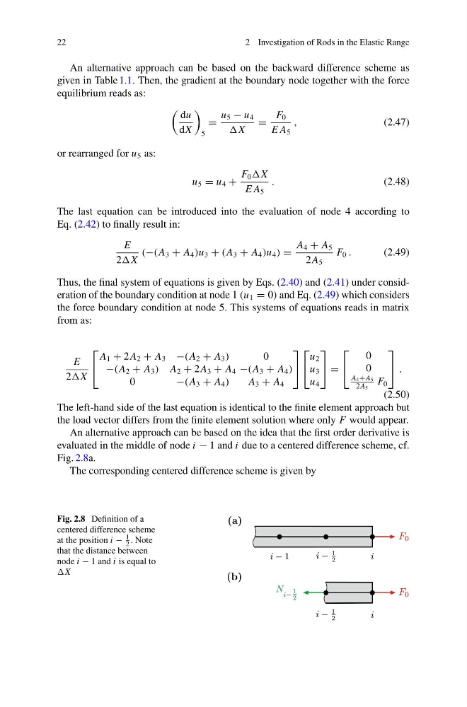
An alternative approach can be based on the idea that the first order derivative is
evaluated in the middle of node i − 1 and i due to a centered difference scheme, cf.
Fig. 2.8a.
The corresponding centered difference scheme is given by
Fig. 2.8 Definition of a
centered difference scheme
at the position i −
1
2 . Note
that the distance between
node i − 1 and i is equal to
2 Investigation of Rods in the Elastic Range
An alternative approach can be based on the backward difference scheme as
given in Table 1.1. Then, the gradient at the boundary node together with the force
equilibrium reads as:
du
dX
5
=
u 5 − u 4
=
F 0
E A 5
,
(2.47)
or rearranged for u 5 as:
u 5 = u 4 +
F 0
E A 5
.
(2.48)
The last equation can be introduced into the evaluation of node 4 according to
Eq. (2.42) to finally result in:
E
2
(−(A 3 + A 4 )u 3 + (A 3 + A 4 )u 4 ) =
A 4 + A 5
2 A 5
F 0 .
(2.49)
Thus, the final system of equations is given by Eqs. (2.40) and (2.41) under consideration of the boundary condition at node 1 (u 1 = 0) and Eq. (2.49) which considers
the force boundary condition at node 5. This systems of equations reads in matrix
from as:
E
2
⎡
⎣
A 1 + 2 A 2 + A 3 −(A 2 + A 3 )
0
−(A 2 + A 3 ) A 2 + 2 A 3 + A 4 −(A 3 + A 4 )
0
−(A 3 + A 4 )
A 3 + A 4
⎤
⎦
⎡
⎣
u 2
u 3
u 4
⎤
⎦ =
⎡
⎣
0
0
A 4 +A 5
2 A 5
F 0
⎤
⎦ .
(2.50)
The left-hand side of the last equation is identical to the finite element approach but
the load vector differs from the finite element solution where only F would appear.
An alternative approach can be based on the idea that the first order derivative is
evaluated in the middle of node i − 1 and i due to a centered difference scheme, cf.
Fig. 2.8a.
The corresponding centered difference scheme is given by
Fig. 2.8 Definition of a
centered difference scheme
at the position i −
1
2 . Note
that the distance between
node i − 1 and i is equal to