

4.2 Approximation of the Differential Equations
95
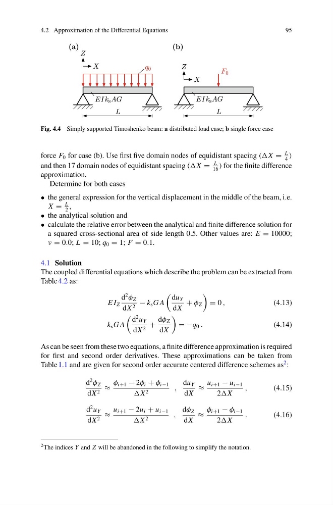
Fig. 4.4 Simply supported Timoshenko beam: a distributed load case; b single force case
force F 0 for case (b). Use first five domain nodes of equidistant spacing ((X =
L
4
)
and then 17 domain nodes of equidistant spacing ((X =
L
16
) for the finite difference
approximation.
Determine for both cases
• the general expression for the vertical displacement in the middle of the beam, i.e.
X =
L
2
,
• the analytical solution and
• calculate the relative error between the analytical and finite difference solution for
a squared cross-sectional area of side length 0.5. Other values are: E = 10000;
ν = 0.0; L = 10; q 0 = 1; F = 0.1.
4.1 Solution
The coupled differential equations which describe the problem can be extracted from
Table 4.2 as:
E I Z
d
2
φ Z
dX 2 − k s G A
du Y
dX
+ φ Z
= 0 ,
(4.13)
k s G A
d
2 u Y
dX 2 +
dφ Z
dX
= −q 0 .
(4.14)
As can be seen from these two equations, a finite difference approximation is required
for first and second order derivatives. These approximations can be taken from
Table 1.1 and are given for second order accurate centered difference schemes as
2 :
d
2
φ Z
dX 2 ≈
φ i+1 − 2φ i + φ i−1
X 2
,
du Y
dX
≈
u i+1 − u i−1
2
,
(4.15)
d
2 u Y
dX 2 ≈
u i+1 − 2u i + u i−1
X 2
,
dφ Z
dX
≈
φ i+1 − φ i−1
2
.
(4.16)
2 The indices Y and Z will be abandoned in the following to simplify the notation.
95
Fig. 4.4 Simply supported Timoshenko beam: a distributed load case; b single force case
force F 0 for case (b). Use first five domain nodes of equidistant spacing ((X =
L
4
)
and then 17 domain nodes of equidistant spacing ((X =
L
16
) for the finite difference
approximation.
Determine for both cases
• the general expression for the vertical displacement in the middle of the beam, i.e.
X =
L
2
,
• the analytical solution and
• calculate the relative error between the analytical and finite difference solution for
a squared cross-sectional area of side length 0.5. Other values are: E = 10000;
ν = 0.0; L = 10; q 0 = 1; F = 0.1.
4.1 Solution
The coupled differential equations which describe the problem can be extracted from
Table 4.2 as:
E I Z
d
2
φ Z
dX 2 − k s G A
du Y
dX
+ φ Z
= 0 ,
(4.13)
k s G A
d
2 u Y
dX 2 +
dφ Z
dX
= −q 0 .
(4.14)
As can be seen from these two equations, a finite difference approximation is required
for first and second order derivatives. These approximations can be taken from
Table 1.1 and are given for second order accurate centered difference schemes as
2 :
d
2
φ Z
dX 2 ≈
φ i+1 − 2φ i + φ i−1
X 2
,
du Y
dX
≈
u i+1 − u i−1
2
,
(4.15)
d
2 u Y
dX 2 ≈
u i+1 − 2u i + u i−1
X 2
,
dφ Z
dX
≈
φ i+1 − φ i−1
2
.
(4.16)
2 The indices Y and Z will be abandoned in the following to simplify the notation.