

96
4 Investigation of Timoshenko Beams in the Elastic Range
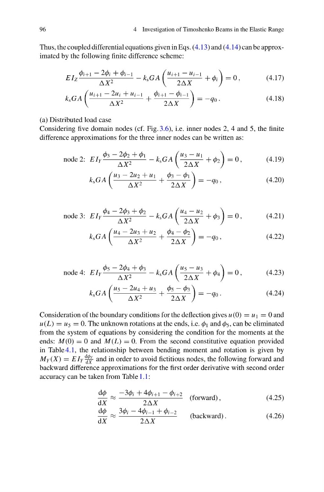
Thus, the coupled differential equations given in Eqs. (4.13) and (4.14) can be approximated by the following finite difference scheme:
E I Z
φ i+1 − 2φ i + φ i−1
X 2
− k s G A
u i+1 − u i−1
2X
+ φ i
= 0 ,
(4.17)
k s G A
u i+1 − 2u i + u i−1
X 2
+
φ i+1 − φ i−1
2X
= −q 0 .
(4.18)
(a) Distributed load case
Considering five domain nodes (cf. Fig. 3.6), i.e. inner nodes 2, 4 and 5, the finite
difference approximations for the three inner nodes can be written as:
node 2: E I Y
φ 3 − 2φ 2 + φ 1
X 2
− k s G A
u 3 − u 1
2X
+ φ 2
= 0 ,
(4.19)
k s G A
u 3 − 2u 2 + u 1
X 2
+
φ 3 − φ 1
2X
= −q 0 ,
(4.20)
node 3: E I Y
φ 4 − 2φ 3 + φ 2
X 2
− k s G A
u 4 − u 2
2X
+ φ 3
= 0 ,
(4.21)
k s G A
u 4 − 2u 3 + u 2
X 2
+
φ 4 − φ 2
2X
= −q 0 ,
(4.22)
node 4: E I Y
φ 5 − 2φ 4 + φ 3
X 2
− k s G A
u 5 − u 3
2X
+ φ 4
= 0 ,
(4.23)
k s G A
u 5 − 2u 4 + u 3
X 2
+
φ 5 − φ 3
2X
= −q 0 .
(4.24)
Consideration of the boundary conditions for the deflection gives u(0) = u 1 = 0 and
u(L) = u 5 = 0. The unknown rotations at the ends, i.e. φ 1 and φ 5 , can be eliminated
from the system of equations by considering the condition for the moments at the
ends: M(0) = 0 and M(L) = 0. From the second constitutive equation provided
in Table 4.1, the relationship between bending moment and rotation is given by
M Y (X ) = E I Y
dφ Y
dX
and in order to avoid fictitious nodes, the following forward and
backward difference approximations for the first order derivative with second order
accuracy can be taken from Table 1.1:
dφ
dX
≈
−3φ i + 4φ i+1 − φ i+2
2X
(forward) ,
(4.25)
dφ
dX
≈
3φ i − 4φ i−1 + φ i−2
2X
(backward) .
(4.26)
4 Investigation of Timoshenko Beams in the Elastic Range
Thus, the coupled differential equations given in Eqs. (4.13) and (4.14) can be approximated by the following finite difference scheme:
E I Z
φ i+1 − 2φ i + φ i−1
X 2
− k s G A
u i+1 − u i−1
2X
+ φ i
= 0 ,
(4.17)
k s G A
u i+1 − 2u i + u i−1
X 2
+
φ i+1 − φ i−1
2X
= −q 0 .
(4.18)
(a) Distributed load case
Considering five domain nodes (cf. Fig. 3.6), i.e. inner nodes 2, 4 and 5, the finite
difference approximations for the three inner nodes can be written as:
node 2: E I Y
φ 3 − 2φ 2 + φ 1
X 2
− k s G A
u 3 − u 1
2X
+ φ 2
= 0 ,
(4.19)
k s G A
u 3 − 2u 2 + u 1
X 2
+
φ 3 − φ 1
2X
= −q 0 ,
(4.20)
node 3: E I Y
φ 4 − 2φ 3 + φ 2
X 2
− k s G A
u 4 − u 2
2X
+ φ 3
= 0 ,
(4.21)
k s G A
u 4 − 2u 3 + u 2
X 2
+
φ 4 − φ 2
2X
= −q 0 ,
(4.22)
node 4: E I Y
φ 5 − 2φ 4 + φ 3
X 2
− k s G A
u 5 − u 3
2X
+ φ 4
= 0 ,
(4.23)
k s G A
u 5 − 2u 4 + u 3
X 2
+
φ 5 − φ 3
2X
= −q 0 .
(4.24)
Consideration of the boundary conditions for the deflection gives u(0) = u 1 = 0 and
u(L) = u 5 = 0. The unknown rotations at the ends, i.e. φ 1 and φ 5 , can be eliminated
from the system of equations by considering the condition for the moments at the
ends: M(0) = 0 and M(L) = 0. From the second constitutive equation provided
in Table 4.1, the relationship between bending moment and rotation is given by
M Y (X ) = E I Y
dφ Y
dX
and in order to avoid fictitious nodes, the following forward and
backward difference approximations for the first order derivative with second order
accuracy can be taken from Table 1.1:
dφ
dX
≈
−3φ i + 4φ i+1 − φ i+2
2X
(forward) ,
(4.25)
dφ
dX
≈
3φ i − 4φ i−1 + φ i−2
2X
(backward) .
(4.26)