

94
4 Investigation of Timoshenko Beams in the Elastic Range
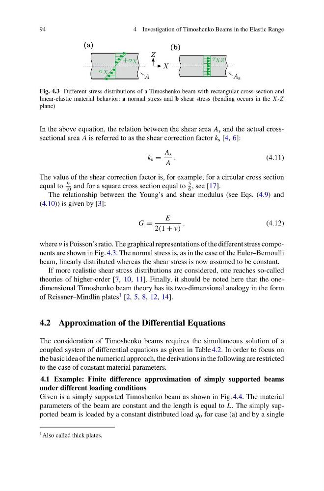
Fig. 4.3 Different stress distributions of a Timoshenko beam with rectangular cross section and
linear-elastic material behavior: a normal stress and b shear stress (bending occurs in the X -Z
plane)
In the above equation, the relation between the shear area A s and the actual crosssectional area A is referred to as the shear correction factor k s [4, 6]:
k s =
A s
A
.
(4.11)
The value of the shear correction factor is, for example, for a circular cross section
equal to
9
10
and for a square cross section equal to
5
6
, see [17].
The relationship between the Young’s and shear modulus (see Eqs. (4.9) and
(4.10)) is given by [3]:
G =
E
2(1 + ν)
,
(4.12)
where ν is Poisson’s ratio. The graphical representations of the different stress components are shown in Fig. 4.3. The normal stress is, as in the case of the Euler–Bernoulli
beam, linearly distributed whereas the shear stress is now assumed to be constant.
If more realistic shear stress distributions are considered, one reaches so-called
theories of higher-order [7, 10, 11]. Finally, it should be noted here that the onedimensional Timoshenko beam theory has its two-dimensional analogy in the form
of Reissner–Mindlin plates
1 [2, 5, 8, 12, 14].
4.2 Approximation of the Differential Equations
The consideration of Timoshenko beams requires the simultaneous solution of a
coupled system of differential equations as given in Table 4.2. In order to focus on
the basic idea of the numerical approach, the derivations in the following are restricted
to the case of constant material parameters.
4.1 Example: Finite difference approximation of simply supported beams
under different loading conditions
Given is a simply supported Timoshenko beam as shown in Fig. 4.4. The material
parameters of the beam are constant and the length is equal to L. The simply supported beam is loaded by a constant distributed load q 0 for case (a) and by a single
1 Also called thick plates.
4 Investigation of Timoshenko Beams in the Elastic Range
Fig. 4.3 Different stress distributions of a Timoshenko beam with rectangular cross section and
linear-elastic material behavior: a normal stress and b shear stress (bending occurs in the X -Z
plane)
In the above equation, the relation between the shear area A s and the actual crosssectional area A is referred to as the shear correction factor k s [4, 6]:
k s =
A s
A
.
(4.11)
The value of the shear correction factor is, for example, for a circular cross section
equal to
9
10
and for a square cross section equal to
5
6
, see [17].
The relationship between the Young’s and shear modulus (see Eqs. (4.9) and
(4.10)) is given by [3]:
G =
E
2(1 + ν)
,
(4.12)
where ν is Poisson’s ratio. The graphical representations of the different stress components are shown in Fig. 4.3. The normal stress is, as in the case of the Euler–Bernoulli
beam, linearly distributed whereas the shear stress is now assumed to be constant.
If more realistic shear stress distributions are considered, one reaches so-called
theories of higher-order [7, 10, 11]. Finally, it should be noted here that the onedimensional Timoshenko beam theory has its two-dimensional analogy in the form
of Reissner–Mindlin plates
1 [2, 5, 8, 12, 14].
4.2 Approximation of the Differential Equations
The consideration of Timoshenko beams requires the simultaneous solution of a
coupled system of differential equations as given in Table 4.2. In order to focus on
the basic idea of the numerical approach, the derivations in the following are restricted
to the case of constant material parameters.
4.1 Example: Finite difference approximation of simply supported beams
under different loading conditions
Given is a simply supported Timoshenko beam as shown in Fig. 4.4. The material
parameters of the beam are constant and the length is equal to L. The simply supported beam is loaded by a constant distributed load q 0 for case (a) and by a single
1 Also called thick plates.