

4.3 Solutions
283
or ΔQ = T ΔS = kT ln ΔW
= (1.38 × 10
−23 )(300) ln 10
8
= 7.626 × 10
−20 J = 0.477 eV
4.58 The Gaussian (normal) distribution is
f (x) =
1
σ
√
2π
e
−(x−μ)
2 /2σ
2
where μ is the mean and σ is the standard deviation. The probability is found
from
(a) P(μ − σ < x < μ + σ ) =
μ+σ
μ−σ
f (x)dx
Letting z =
x−μ
σ
P(−1 < z < 1) =
1
−1
φ(z)dz
= 2
1
0
φ(z)dz (from symmetry)
= 2 × 0.3413 = 0.6826 (from tables)
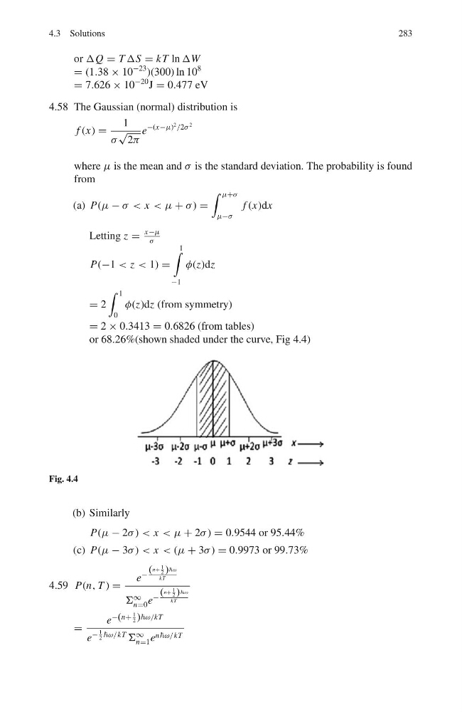
or 68.26%(shown shaded under the curve, Fig 4.4)
Fig. 4.4
(b) Similarly
P(μ − 2σ ) < x < μ + 2σ ) = 0.9544 or 95.44%
(c) P(μ − 3σ ) < x < (μ + 3σ ) = 0.9973 or 99.73%
4.59 P(n, T ) =
e
−
( n+ 1
2 ) ω
kT
Σ
∞
n=0 e
−
( n+ 1
2 ) ω
kT
=
e
−(n+
1
2 )ω/kT
e
−
1
2 ω/kT
Σ
∞
n=1 e nω/kT
283
or ΔQ = T ΔS = kT ln ΔW
= (1.38 × 10
−23 )(300) ln 10
8
= 7.626 × 10
−20 J = 0.477 eV
4.58 The Gaussian (normal) distribution is
f (x) =
1
σ
√
2π
e
−(x−μ)
2 /2σ
2
where μ is the mean and σ is the standard deviation. The probability is found
from
(a) P(μ − σ < x < μ + σ ) =
μ+σ
μ−σ
f (x)dx
Letting z =
x−μ
σ
P(−1 < z < 1) =
1
−1
φ(z)dz
= 2
1
0
φ(z)dz (from symmetry)
= 2 × 0.3413 = 0.6826 (from tables)
or 68.26%(shown shaded under the curve, Fig 4.4)
Fig. 4.4
(b) Similarly
P(μ − 2σ ) < x < μ + 2σ ) = 0.9544 or 95.44%
(c) P(μ − 3σ ) < x < (μ + 3σ ) = 0.9973 or 99.73%
4.59 P(n, T ) =
e
−
( n+ 1
2 ) ω
kT
Σ
∞
n=0 e
−
( n+ 1
2 ) ω
kT
=
e
−(n+
1
2 )ω/kT
e
−
1
2 ω/kT
Σ
∞
n=1 e nω/kT