

242
3 Quantum Mechanics – II
But the total cross-section is given by
σ t =
4π
k 2 (2l + 1) sin
2
δ l .
It follows that I m f (0) = kσ t /4π. The last equation is known as the optical theorem.
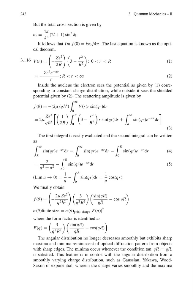
3.116 V (r ) =
−
Ze
2
2R
3 −
r
2
R 2
; 0 < r < R
(1)
= −
Ze
2 e
−ar
r
; R < r < ∞
(2)
Inside the nucleus the electron sees the potential as given by (1) corresponding to constant charge distribution, while outside it sees the shielded
potential given by (2). The scattering amplitude is given by
f (θ ) = −(2μ/q
2 )
∞
0
V (r )r sin(qr )dr
= 2μ
Ze
2
q 2
1
2R
R
0
3 −
r
2
R 2
r sin(qr )dr +
∞
R
sin(qr )e
−ar dr
(3)
The first integral is easily evaluated and the second integral can be written
as
∞
R
sin(qr )e
−ar dr =
∞
0
sin(qr )e
−ar dr −
R
0
sin(qr )e
−ar dr
(4)
=
q
q 2 + a 2 −
R
0
sin(qr )e
−ar dr
(5)
(Lim a → 0) =
1
q
−
R
0
sin(qr)dr =
1
q
cos(qr)
We finally obtain
f (θ ) =
−
2μZe
2
q 2 2
3
q 2 R 2
sin(qR)
qR
− cos qR
σ (θ )finite size = σ (θ ) point charge |F(q)|
2
where the form factor is identified as
F(q) =
3
q 2 R 2
sin(qR)
qR
− cos(qR)
The angular distribution no longer decreases smoothly but exhibits sharp
maxima and minima reminiscent of optical diffraction pattern from objects
with sharp edges. The minima occur whenever the condition tan qR = qR,
is satisfied. This feature is in contrst with the angular distribution from a
smoothly varying charge distribution, such as Gaussian, Yakawa, WoodSaxon or exponential, wherein the charge varies smoothly and the maxima
3 Quantum Mechanics – II
But the total cross-section is given by
σ t =
4π
k 2 (2l + 1) sin
2
δ l .
It follows that I m f (0) = kσ t /4π. The last equation is known as the optical theorem.
3.116 V (r ) =
−
Ze
2
2R
3 −
r
2
R 2
; 0 < r < R
(1)
= −
Ze
2 e
−ar
r
; R < r < ∞
(2)
Inside the nucleus the electron sees the potential as given by (1) corresponding to constant charge distribution, while outside it sees the shielded
potential given by (2). The scattering amplitude is given by
f (θ ) = −(2μ/q
2 )
∞
0
V (r )r sin(qr )dr
= 2μ
Ze
2
q 2
1
2R
R
0
3 −
r
2
R 2
r sin(qr )dr +
∞
R
sin(qr )e
−ar dr
(3)
The first integral is easily evaluated and the second integral can be written
as
∞
R
sin(qr )e
−ar dr =
∞
0
sin(qr )e
−ar dr −
R
0
sin(qr )e
−ar dr
(4)
=
q
q 2 + a 2 −
R
0
sin(qr )e
−ar dr
(5)
(Lim a → 0) =
1
q
−
R
0
sin(qr)dr =
1
q
cos(qr)
We finally obtain
f (θ ) =
−
2μZe
2
q 2 2
3
q 2 R 2
sin(qR)
qR
− cos qR
σ (θ )finite size = σ (θ ) point charge |F(q)|
2
where the form factor is identified as
F(q) =
3
q 2 R 2
sin(qR)
qR
− cos(qR)
The angular distribution no longer decreases smoothly but exhibits sharp
maxima and minima reminiscent of optical diffraction pattern from objects
with sharp edges. The minima occur whenever the condition tan qR = qR,
is satisfied. This feature is in contrst with the angular distribution from a
smoothly varying charge distribution, such as Gaussian, Yakawa, WoodSaxon or exponential, wherein the charge varies smoothly and the maxima