

III.4. Conditions de minimalité du second ordre
Commentaire : Cette manière de transformer des contraintes du type égalité et
inégalité en contraintes du type égalité exclusivement est appelée parfois transformation de Valentine (non non, ce n’est pas le prénom de l’étudiante voisine,
mais le nom d’un mathématicien du XX e siècle qui a travaillé sur les problèmes
variationnels).
Solution : On définit les fonctions ˆ
f, ˆ
h 1 , . . . , ˆ
h m+p : R n × R p → R comme
suit :
∀ (x, y) ∈ R
n
× R
p , ˆ
f (x, y) := f (x),
ˆ
h i (x, y) := h i (x) pour i = 1, . . . , m,
ˆ
h m+j (x, y) := g j (x) + y
2
j pour j = 1, . . . , p.
1 ◦ ) Pour x ∈ S considérons (y 1 , . . . , y p ) ∈ R p tel que ˆ
h m+j (x, y) =
g j (x) + y 2
j = 0 pour j = 1, . . . , p. Notons que y j = 0 exactement pour les
j ∈ J (x) . L’implication suivante est alors claire :
⎛
⎜
⎝
x est un minimum
local de f sur S
⎞
⎟
⎠ ⇒
⎛
⎜
⎜
⎝
(x, y) est un minimum local de ˆ
f sur
ˆ
S :=
(x, y) ∈ R n × R p | ˆ
h k (x, y) = 0
pour k = 1, . . . , m + p}
⎞
⎟
⎟
⎠ .
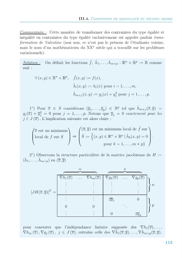
2 ◦ ) Observons la structure particulière de la matrice jacobienne de H :=
( ˆ
h 1 , . . . , ˆ
h m+p ) en (x, y)
[JH(x, y)]
T =
m
p
∇h 1 (x) . . . ∇h m (x) ∇g 1 (x) . . . ∇g p (x)
. . .
. . .
. . .
. . .
. . .
. . .
. . .
. . .
. . .
. . .
2y 1
0
0
0
. . .
. . .
. . .
0
2y p
⎫
⎬
⎭
n
⎫
⎬
⎭
p
pour constater que l’indépendance linéaire supposée des ∇h 1 (x), . . . ,
∇h m (x) , ∇g j (x) , j ∈ J (x), entraîne celle des ∇ ˆ
h 1 (x, y), . . . , ∇ ˆ
h m+p (x, y).
113
Commentaire : Cette manière de transformer des contraintes du type égalité et
inégalité en contraintes du type égalité exclusivement est appelée parfois transformation de Valentine (non non, ce n’est pas le prénom de l’étudiante voisine,
mais le nom d’un mathématicien du XX e siècle qui a travaillé sur les problèmes
variationnels).
Solution : On définit les fonctions ˆ
f, ˆ
h 1 , . . . , ˆ
h m+p : R n × R p → R comme
suit :
∀ (x, y) ∈ R
n
× R
p , ˆ
f (x, y) := f (x),
ˆ
h i (x, y) := h i (x) pour i = 1, . . . , m,
ˆ
h m+j (x, y) := g j (x) + y
2
j pour j = 1, . . . , p.
1 ◦ ) Pour x ∈ S considérons (y 1 , . . . , y p ) ∈ R p tel que ˆ
h m+j (x, y) =
g j (x) + y 2
j = 0 pour j = 1, . . . , p. Notons que y j = 0 exactement pour les
j ∈ J (x) . L’implication suivante est alors claire :
⎛
⎜
⎝
x est un minimum
local de f sur S
⎞
⎟
⎠ ⇒
⎛
⎜
⎜
⎝
(x, y) est un minimum local de ˆ
f sur
ˆ
S :=
(x, y) ∈ R n × R p | ˆ
h k (x, y) = 0
pour k = 1, . . . , m + p}
⎞
⎟
⎟
⎠ .
2 ◦ ) Observons la structure particulière de la matrice jacobienne de H :=
( ˆ
h 1 , . . . , ˆ
h m+p ) en (x, y)
[JH(x, y)]
T =
m
p
∇h 1 (x) . . . ∇h m (x) ∇g 1 (x) . . . ∇g p (x)
. . .
. . .
. . .
. . .
. . .
. . .
. . .
. . .
. . .
. . .
2y 1
0
0
0
. . .
. . .
. . .
0
2y p
⎫
⎬
⎭
n
⎫
⎬
⎭
p
pour constater que l’indépendance linéaire supposée des ∇h 1 (x), . . . ,
∇h m (x) , ∇g j (x) , j ∈ J (x), entraîne celle des ∇ ˆ
h 1 (x, y), . . . , ∇ ˆ
h m+p (x, y).
113