

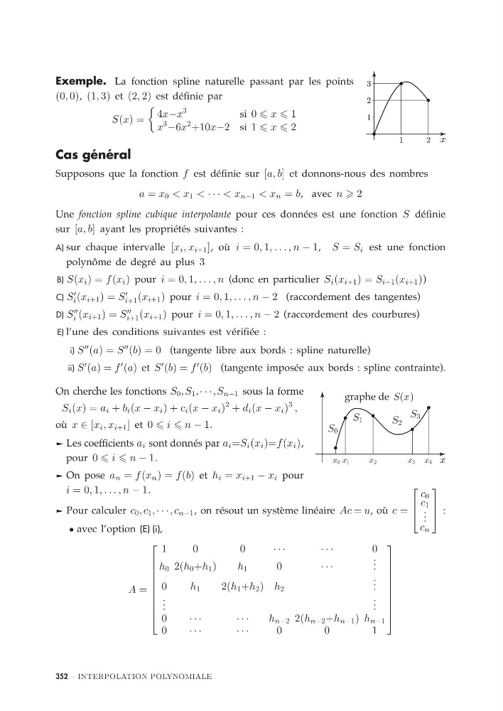
Exemple.
1
2
1
2
3
x
La fonction spline naturelle passant par les points
(0, 0), (1, 3) et (2, 2) est définie par
S(x) =
4x−x
3
si 0 x 1
x
3
−6x
2 +10x−2 si 1 x 2
Cas général
Supposons que la fonction f est définie sur [a, b] et donnons-nous des nombres
a = x 0 < x 1 < · · · < x n−1 < x n = b, avec n 2
Une fonction spline cubique interpolante pour ces données est une fonction S définie
sur [a, b] ayant les propriétés suivantes :
A) sur chaque intervalle [x i , x i+1 ], où i = 0, 1, . . . , n − 1, S = S i est une fonction
polynôme de degré au plus 3
B) S(x i ) = f (x i ) pour i = 0, 1, . . . , n (donc en particulier S i (x i+1 ) = S i+1 (x i+1 ))
C) S
i (x i+1 ) = S
i+1 (x i+1 ) pour i = 0, 1, . . . , n − 2 (raccordement des tangentes)
D) S
i (x i+1 ) = S
i+1 (x i+1 ) pour i = 0, 1, . . . , n − 2 (raccordement des courbures)
E) l’une des conditions suivantes est vérifiée :
i) S
(a) = S
(b) = 0 (tangente libre aux bords : spline naturelle)
ii) S
(a) = f
(a) et S
(b) = f
(b) (tangente imposée aux bords : spline contrainte).
graphe de S(x)
1
0
2
3
4
S 0
S 1
S 2
S 3
x
x
x
x x x
On cherche les fonctions S 0 ,S 1 ,· · ·,S n−1 sous la forme
S i (x) = a i + b i (x − x i ) + c i (x − x i )
2 + d i (x − x i )
3 ,
où x ∈ [x i , x i+1 ] et 0 i n − 1.
® Les coefficients a i sont donnés par a i =S i (x i )=f (x i ),
pour 0 i n − 1.
® On pose a n = f (x n ) = f (b) et h i = x i+1 − x i pour
i = 0, 1, . . . , n − 1.
® Pour calculer c 0 , c 1 , · · ·, c n−1 , on résout un système linéaire Ac = u, où c =
⎡
⎢
⎣
c 0
c 1
. . .
c n
⎤
⎥
⎦ :
• avec l’option (E) (i),
A =
⎡
⎢
⎢
⎢
⎢
⎢
⎢
⎢
⎢
⎣
1
0
0
· · ·
· · ·
0
h 0 2(h 0 +h 1 )
h 1
0
· · ·
. . .
0
h 1
2(h 1 +h 2 ) h 2
. . .
. . .
. . .
0
· · ·
· · ·
h n−2 2(h n−2 +h n−1 ) h n−1
0
· · ·
· · ·
0
0
1
⎤
⎥
⎥
⎥
⎥
⎥
⎥
⎥
⎥
⎦
352 – INTERPOLATION POLYNOMIALE
1
2
1
2
3
x
La fonction spline naturelle passant par les points
(0, 0), (1, 3) et (2, 2) est définie par
S(x) =
4x−x
3
si 0 x 1
x
3
−6x
2 +10x−2 si 1 x 2
Cas général
Supposons que la fonction f est définie sur [a, b] et donnons-nous des nombres
a = x 0 < x 1 < · · · < x n−1 < x n = b, avec n 2
Une fonction spline cubique interpolante pour ces données est une fonction S définie
sur [a, b] ayant les propriétés suivantes :
A) sur chaque intervalle [x i , x i+1 ], où i = 0, 1, . . . , n − 1, S = S i est une fonction
polynôme de degré au plus 3
B) S(x i ) = f (x i ) pour i = 0, 1, . . . , n (donc en particulier S i (x i+1 ) = S i+1 (x i+1 ))
C) S
i (x i+1 ) = S
i+1 (x i+1 ) pour i = 0, 1, . . . , n − 2 (raccordement des tangentes)
D) S
i (x i+1 ) = S
i+1 (x i+1 ) pour i = 0, 1, . . . , n − 2 (raccordement des courbures)
E) l’une des conditions suivantes est vérifiée :
i) S
(a) = S
(b) = 0 (tangente libre aux bords : spline naturelle)
ii) S
(a) = f
(a) et S
(b) = f
(b) (tangente imposée aux bords : spline contrainte).
graphe de S(x)
1
0
2
3
4
S 0
S 1
S 2
S 3
x
x
x
x x x
On cherche les fonctions S 0 ,S 1 ,· · ·,S n−1 sous la forme
S i (x) = a i + b i (x − x i ) + c i (x − x i )
2 + d i (x − x i )
3 ,
où x ∈ [x i , x i+1 ] et 0 i n − 1.
® Les coefficients a i sont donnés par a i =S i (x i )=f (x i ),
pour 0 i n − 1.
® On pose a n = f (x n ) = f (b) et h i = x i+1 − x i pour
i = 0, 1, . . . , n − 1.
® Pour calculer c 0 , c 1 , · · ·, c n−1 , on résout un système linéaire Ac = u, où c =
⎡
⎢
⎣
c 0
c 1
. . .
c n
⎤
⎥
⎦ :
• avec l’option (E) (i),
A =
⎡
⎢
⎢
⎢
⎢
⎢
⎢
⎢
⎢
⎣
1
0
0
· · ·
· · ·
0
h 0 2(h 0 +h 1 )
h 1
0
· · ·
. . .
0
h 1
2(h 1 +h 2 ) h 2
. . .
. . .
. . .
0
· · ·
· · ·
h n−2 2(h n−2 +h n−1 ) h n−1
0
· · ·
· · ·
0
0
1
⎤
⎥
⎥
⎥
⎥
⎥
⎥
⎥
⎥
⎦
352 – INTERPOLATION POLYNOMIALE