

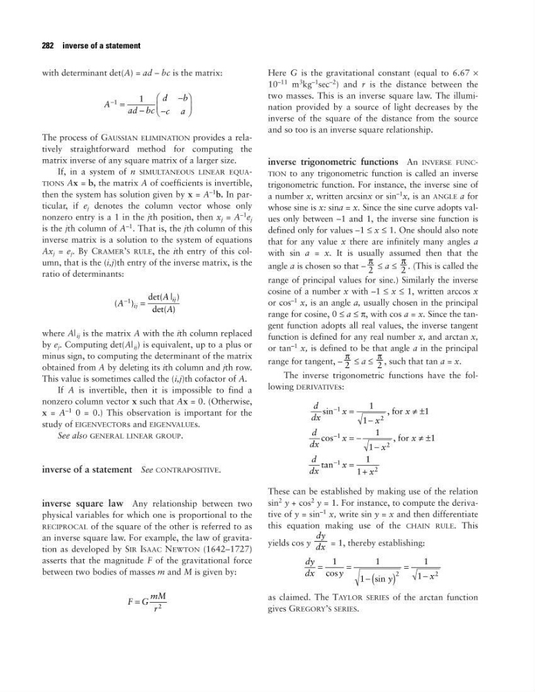
with determinant det(A) = ad – bc is the matrix:
The process of GAUSSIAN ELIMINATION provides a relatively straightforward method for computing the
matrix inverse of any square matrix of a larger size.
If, in a system of n SIMULTANEOUS LINEAR EQUATIONS Ax = b, the matrix A of coefficients is invertible,
then the system has solution given by x = A
–1 b. In particular, if e j denotes the column vector whose only
nonzero entry is a 1 in the jth position, then x j = A
–1 e j
is the jth column of A
–1 . That is, the jth column of this
inverse matrix is a solution to the system of equations
Ax j = e j . By CRAMER’S RULE, the ith entry of this column, that is the (i,j)th entry of the inverse matrix, is the
ratio of determinants:
where A| ij is the matrix A with the ith column replaced
by e j . Computing det(A| ij ) is equivalent, up to a plus or
minus sign, to computing the determinant of the matrix
obtained from A by deleting its ith column and jth row.
This value is sometimes called the (i,j)th cofactor of A.
If A is invertible, then it is impossible to find a
nonzero column vector x such that Ax = 0. (Otherwise,
x = A
–1 0 = 0.) This observation is important for the
study of EIGENVECTORs and EIGENVALUEs.
See also GENERAL LINEAR GROUP.
inverse of a statement See CONTRAPOSITIVE.
inverse square law Any relationship between two
physical variables for which one is proportional to the
RECIPROCAL of the square of the other is referred to as
an inverse square law. For example, the law of gravitation as developed by SIR ISAAC NEWTON (1642–1727)
asserts that the magnitude F of the gravitational force
between two bodies of masses m and M is given by:
Here G is the gravitational constant (equal to 6.67 ×
10
–11 m
3 kg
–1 sec
–2 ) and r is the distance between the
two masses. This is an inverse square law. The illumination provided by a source of light decreases by the
inverse of the square of the distance from the source
and so too is an inverse square relationship.
inverse trigonometric functions An INVERSE FUNCTION to any trigonometric function is called an inverse
trigonometric function. For instance, the inverse sine of
a number x, written arcsinx or sin
–1
x, is an ANGLE a for
whose sine is x: sina = x. Since the sine curve adopts values only between –1 and 1, the inverse sine function is
defined only for values –1 ≤ x ≤ 1. One should also note
that for any value x there are infinitely many angles a
with sin a = x. It is usually assumed then that the
angle a is chosen so that – ≤ a ≤ . (This is called the
range of principal values for sine.) Similarly the inverse
cosine of a number x with –1 ≤ x ≤ 1, written arccos x
or cos
–1 x, is an angle a, usually chosen in the principal
range for cosine, 0 ≤ a ≤ π, with cos a = x. Since the tangent function adopts all real values, the inverse tangent
function is defined for any real number x, and arctan x,
or tan
–1 x, is defined to be that angle a in the principal
range for tangent, – ≤ a ≤ , such that tan a = x.
The inverse trigonometric functions have the following DERIVATIVEs:
These can be established by making use of the relation
sin
2 y + cos
2 y = 1. For instance, to compute the derivative of y = sin
–1 x, write sin y = x and then differentiate
this equation making use of the CHAIN RULE. This
yields cos y
= 1, thereby establishing:
as claimed. The TAYLOR SERIES of the arctan function
gives GREGORY’S SERIES.
dy
dx
y
y
x
=
=
− ( )
=
−
1
1
1
1
1
2
2
cos
sin
dy
––
dx
d
dx
x
x
x
d
dx
x
x
x
d
dx
x
x
sin
,
cos
,
tan
−
−
−
=
−
≠ ±
= −
−
≠ ±
= +
1
2
1
2
1
2
1
1
1
1
1
1
1
1
for
for
π
–
2
π
–
2
π
–
2
π
–
2
F G
mM
r
=
2
(
)
det( | )
det( )
A
A
A
ij
ij
−
=
1
A
ad bc
d
b
c a
−
=
−
−
−
1
1
282 inverse of a statement
The process of GAUSSIAN ELIMINATION provides a relatively straightforward method for computing the
matrix inverse of any square matrix of a larger size.
If, in a system of n SIMULTANEOUS LINEAR EQUATIONS Ax = b, the matrix A of coefficients is invertible,
then the system has solution given by x = A
–1 b. In particular, if e j denotes the column vector whose only
nonzero entry is a 1 in the jth position, then x j = A
–1 e j
is the jth column of A
–1 . That is, the jth column of this
inverse matrix is a solution to the system of equations
Ax j = e j . By CRAMER’S RULE, the ith entry of this column, that is the (i,j)th entry of the inverse matrix, is the
ratio of determinants:
where A| ij is the matrix A with the ith column replaced
by e j . Computing det(A| ij ) is equivalent, up to a plus or
minus sign, to computing the determinant of the matrix
obtained from A by deleting its ith column and jth row.
This value is sometimes called the (i,j)th cofactor of A.
If A is invertible, then it is impossible to find a
nonzero column vector x such that Ax = 0. (Otherwise,
x = A
–1 0 = 0.) This observation is important for the
study of EIGENVECTORs and EIGENVALUEs.
See also GENERAL LINEAR GROUP.
inverse of a statement See CONTRAPOSITIVE.
inverse square law Any relationship between two
physical variables for which one is proportional to the
RECIPROCAL of the square of the other is referred to as
an inverse square law. For example, the law of gravitation as developed by SIR ISAAC NEWTON (1642–1727)
asserts that the magnitude F of the gravitational force
between two bodies of masses m and M is given by:
Here G is the gravitational constant (equal to 6.67 ×
10
–11 m
3 kg
–1 sec
–2 ) and r is the distance between the
two masses. This is an inverse square law. The illumination provided by a source of light decreases by the
inverse of the square of the distance from the source
and so too is an inverse square relationship.
inverse trigonometric functions An INVERSE FUNCTION to any trigonometric function is called an inverse
trigonometric function. For instance, the inverse sine of
a number x, written arcsinx or sin
–1
x, is an ANGLE a for
whose sine is x: sina = x. Since the sine curve adopts values only between –1 and 1, the inverse sine function is
defined only for values –1 ≤ x ≤ 1. One should also note
that for any value x there are infinitely many angles a
with sin a = x. It is usually assumed then that the
angle a is chosen so that – ≤ a ≤ . (This is called the
range of principal values for sine.) Similarly the inverse
cosine of a number x with –1 ≤ x ≤ 1, written arccos x
or cos
–1 x, is an angle a, usually chosen in the principal
range for cosine, 0 ≤ a ≤ π, with cos a = x. Since the tangent function adopts all real values, the inverse tangent
function is defined for any real number x, and arctan x,
or tan
–1 x, is defined to be that angle a in the principal
range for tangent, – ≤ a ≤ , such that tan a = x.
The inverse trigonometric functions have the following DERIVATIVEs:
These can be established by making use of the relation
sin
2 y + cos
2 y = 1. For instance, to compute the derivative of y = sin
–1 x, write sin y = x and then differentiate
this equation making use of the CHAIN RULE. This
yields cos y
= 1, thereby establishing:
as claimed. The TAYLOR SERIES of the arctan function
gives GREGORY’S SERIES.
dy
dx
y
y
x
=
=
− ( )
=
−
1
1
1
1
1
2
2
cos
sin
dy
––
dx
d
dx
x
x
x
d
dx
x
x
x
d
dx
x
x
sin
,
cos
,
tan
−
−
−
=
−
≠ ±
= −
−
≠ ±
= +
1
2
1
2
1
2
1
1
1
1
1
1
1
1
for
for
π
–
2
π
–
2
π
–
2
π
–
2
F G
mM
r
=
2
(
)
det( | )
det( )
A
A
A
ij
ij
−
=
1
A
ad bc
d
b
c a
−
=
−
−
−
1
1
282 inverse of a statement