

Consequences for Matrix Theory
Any system of linear equations can be represented via a
coefficient MATRIX and a column of constant values.
For instance, for our example:
y + 3z = 0
2x + 4y – 2z = 18
x + 5y + 3z = 14
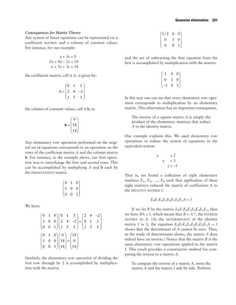
the coefficient matrix, call it A, is given by:
the column of constant values, call it b, is:
Any elementary row operation performed on the original set of equations corresponds to an operation on the
rows of the coefficient matrix A and the column matrix
b. For instance, in the example above, our first operation was to interchange the first and second rows. This
can be accomplished by multiplying A and b each by
the PERMUTATION matrix
We have:
Similarly, the elementary row operation of dividing the
first row through by 2 is accomplished by multiplication with the matrix
and the act of subtracting the first equation from the
first is accomplished by multiplication with the matrix:
In this way one can see that every elementary row operation corresponds to multiplication by an elementary
matrix. This observation has an important consequence.
The inverse of a square matrix A is simply the
product of the elementary matrices that reduce
A to the identity matrix.
Our example explains this. We used elementary row
operations to reduce the system of equations to the
equivalent system:
x
= 2
y = 3
z = –1
That is, we found a collection of eight elementary
matrices E 1 , E 2 , …, E 8 such that application of these
eight matrices reduced the matrix of coefficients A to
the IDENTITY MATRIX I.
E 8 E 7 E 6 E 5 E 4 E 3 E 2 E 1 A = I
If we let B be the matrix E 8 E 7 E 6 E 5 E 4 E 3 E 2 E 1 , then
we have BA = I, which means that B = A
–1 , the INVERSE
MATRIX to A. (As the DETERMINANT of the identity
matrix I is 1, the equation E 8 E 7 E 6 E 5 E 4 E 3 E 2 E 1 A = I
shows that the determinant of A cannot be zero. Thus,
as the study of determinants shows, the matrix A does
indeed have an inverse.) Notice that the matrix B is the
same elementary row operations applied to the matrix
I. This result provides a constructive method for computing the inverse to a matrix A.
To compute the inverse of a matrix A, write the
matrix A and the matrix I side by side. Perform
1 0 0
0 1 0
1 0 1
−
1 2 0 0
0 1 0
0 0 1
/
0 1 0
1 0 0
0 0 1
0 1 3
2 4 2
1 5 3
2 4 2
0 1 3
1 5 3
0 1 0
1 0 0
0 0 1
0
18
14
18
0
14
−
=
−
=
0 1 0
1 0 0
0 0 1
b =
0
18
14
A =
−
0 1 3
2 4 2
1 5 3
Gaussian elimination 221
Any system of linear equations can be represented via a
coefficient MATRIX and a column of constant values.
For instance, for our example:
y + 3z = 0
2x + 4y – 2z = 18
x + 5y + 3z = 14
the coefficient matrix, call it A, is given by:
the column of constant values, call it b, is:
Any elementary row operation performed on the original set of equations corresponds to an operation on the
rows of the coefficient matrix A and the column matrix
b. For instance, in the example above, our first operation was to interchange the first and second rows. This
can be accomplished by multiplying A and b each by
the PERMUTATION matrix
We have:
Similarly, the elementary row operation of dividing the
first row through by 2 is accomplished by multiplication with the matrix
and the act of subtracting the first equation from the
first is accomplished by multiplication with the matrix:
In this way one can see that every elementary row operation corresponds to multiplication by an elementary
matrix. This observation has an important consequence.
The inverse of a square matrix A is simply the
product of the elementary matrices that reduce
A to the identity matrix.
Our example explains this. We used elementary row
operations to reduce the system of equations to the
equivalent system:
x
= 2
y = 3
z = –1
That is, we found a collection of eight elementary
matrices E 1 , E 2 , …, E 8 such that application of these
eight matrices reduced the matrix of coefficients A to
the IDENTITY MATRIX I.
E 8 E 7 E 6 E 5 E 4 E 3 E 2 E 1 A = I
If we let B be the matrix E 8 E 7 E 6 E 5 E 4 E 3 E 2 E 1 , then
we have BA = I, which means that B = A
–1 , the INVERSE
MATRIX to A. (As the DETERMINANT of the identity
matrix I is 1, the equation E 8 E 7 E 6 E 5 E 4 E 3 E 2 E 1 A = I
shows that the determinant of A cannot be zero. Thus,
as the study of determinants shows, the matrix A does
indeed have an inverse.) Notice that the matrix B is the
same elementary row operations applied to the matrix
I. This result provides a constructive method for computing the inverse to a matrix A.
To compute the inverse of a matrix A, write the
matrix A and the matrix I side by side. Perform
1 0 0
0 1 0
1 0 1
−
1 2 0 0
0 1 0
0 0 1
/
0 1 0
1 0 0
0 0 1
0 1 3
2 4 2
1 5 3
2 4 2
0 1 3
1 5 3
0 1 0
1 0 0
0 0 1
0
18
14
18
0
14
−
=
−
=
0 1 0
1 0 0
0 0 1
b =
0
18
14
A =
−
0 1 3
2 4 2
1 5 3
Gaussian elimination 221