

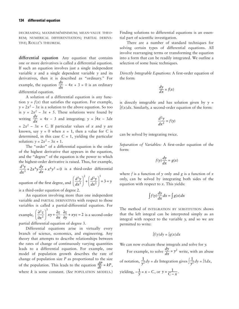
DECREASING; MAXIMUM/MINIMUM; MEAN-VALUE THEOREM; NUMERICAL DIFFERENTIATION; PARTIAL DERIVATIVE; ROLLE’S THEOREM.
differential equation Any equation that contains
one or more derivatives is called a differential equation.
If such an equation involves just a single independent
variable x and a single dependent variable y and its
derivatives, then it is described as “ordinary.” For
example, the equation
– 4x + 3 = 0 is an ordinary
differential equation.
A solution of a differential equation is any function y = f(x) that satisfies the equation. For example,
y = 2x
2 – 3x is a solution to the above equation. So too
is y = 2x
2 – 3x + 5. These solutions were found by
writing
= 4x – 3 and integrating: y = ∫4x – 3dx
= 2x
2 – 3x + C. If particular values of x and y are
known, say y = 0 when x = 1, then a value for C is
determined, in this case C = 1, yielding the particular
solution: y = 2x
2 – 3x + 1.
The “order” of a differential equation is the order
of the highest derivative that appears in the equation,
and the “degree” of the equation is the power to which
the highest-order derivative is raised. Thus, for example,
is a third-order differential
equation of the first degree, and
is a third-order equation of degree 2.
An equation involving more than one independent
variable and PARTIAL DERIVATIVEs with respect to those
variables is called a partial-differential equation. For
example,
is a second-order
partial differential equation of degree 3.
Differential equations arise in virtually every
branch of science, economics, and engineering. Any
theory that attempts to describe relationships between
the rates of change of continuously varying quantities
leads to a differential equation. For example, one
model of population growth describes the rate of
change of population size P as proportional to the size
of the population. This leads to the equation
,
where k is some constant. (See POPULATION MODELS.)
Finding solutions to differential equations is an essential part of scientific investigation.
There are a number of standard techniques for
solving certain types of differential equations. All
involve rearranging terms or transforming the equation
into a form that can be readily integrated. We outline a
selection of some basic techniques.
Directly Integrable Equations: A first-order equation of
the form:
is directly integrable and has solution given by y =
∫f(x)dx. Similarly, a second-order equation of the form:
can be solved by integrating twice.
Separation of Variables: A first-order equation of the
form:
where f is a function of y only and g is a function of x
only, can be solved by integrating both sides of the
equation with respect to x. This yields:
The method of INTEGRATION BY SUBSTITUTION shows
that the left integral can be interpreted simply as an
integral with respect to the variable y, and so we are
permitted to write:
∫f(y)dy = ∫g(x)dx
We can now evaluate these integrals and solve for y.
For example, to solve
write, with an abuse
of notation, dy = dx Integration gives ∫ dy = ∫1dx,
yielding,
, or
.
1
y = ——–
C – x
1
– – = x – C
y
1
–
y
2
1
–
y
2
dy
–– = y
2
dx
f y
dy
dx
dx
g x dx
( )
( )
∫
∫
=
f y
dy
dx
g x
( )
( )
=
d y
dx
f y
2
2
= ( )
dy
–– = f(x)
dx
dP –– = kP
dt
∂
∂
+
∂
∂
⋅
∂
∂
+
=
2
2
3
2
z
x
xy
z
x
z
y
xyz
d y
dx
d y
dx
y
3
3
2
2
2
5
3
+
+ =
d y
dx
x y
dy
dx
x y
3
3
4
6 2
2
0
+
+
=
dy
––
dx
dy
––
dx
134 differential equation
differential equation Any equation that contains
one or more derivatives is called a differential equation.
If such an equation involves just a single independent
variable x and a single dependent variable y and its
derivatives, then it is described as “ordinary.” For
example, the equation
– 4x + 3 = 0 is an ordinary
differential equation.
A solution of a differential equation is any function y = f(x) that satisfies the equation. For example,
y = 2x
2 – 3x is a solution to the above equation. So too
is y = 2x
2 – 3x + 5. These solutions were found by
writing
= 4x – 3 and integrating: y = ∫4x – 3dx
= 2x
2 – 3x + C. If particular values of x and y are
known, say y = 0 when x = 1, then a value for C is
determined, in this case C = 1, yielding the particular
solution: y = 2x
2 – 3x + 1.
The “order” of a differential equation is the order
of the highest derivative that appears in the equation,
and the “degree” of the equation is the power to which
the highest-order derivative is raised. Thus, for example,
is a third-order differential
equation of the first degree, and
is a third-order equation of degree 2.
An equation involving more than one independent
variable and PARTIAL DERIVATIVEs with respect to those
variables is called a partial-differential equation. For
example,
is a second-order
partial differential equation of degree 3.
Differential equations arise in virtually every
branch of science, economics, and engineering. Any
theory that attempts to describe relationships between
the rates of change of continuously varying quantities
leads to a differential equation. For example, one
model of population growth describes the rate of
change of population size P as proportional to the size
of the population. This leads to the equation
,
where k is some constant. (See POPULATION MODELS.)
Finding solutions to differential equations is an essential part of scientific investigation.
There are a number of standard techniques for
solving certain types of differential equations. All
involve rearranging terms or transforming the equation
into a form that can be readily integrated. We outline a
selection of some basic techniques.
Directly Integrable Equations: A first-order equation of
the form:
is directly integrable and has solution given by y =
∫f(x)dx. Similarly, a second-order equation of the form:
can be solved by integrating twice.
Separation of Variables: A first-order equation of the
form:
where f is a function of y only and g is a function of x
only, can be solved by integrating both sides of the
equation with respect to x. This yields:
The method of INTEGRATION BY SUBSTITUTION shows
that the left integral can be interpreted simply as an
integral with respect to the variable y, and so we are
permitted to write:
∫f(y)dy = ∫g(x)dx
We can now evaluate these integrals and solve for y.
For example, to solve
write, with an abuse
of notation, dy = dx Integration gives ∫ dy = ∫1dx,
yielding,
, or
.
1
y = ——–
C – x
1
– – = x – C
y
1
–
y
2
1
–
y
2
dy
–– = y
2
dx
f y
dy
dx
dx
g x dx
( )
( )
∫
∫
=
f y
dy
dx
g x
( )
( )
=
d y
dx
f y
2
2
= ( )
dy
–– = f(x)
dx
dP –– = kP
dt
∂
∂
+
∂
∂
⋅
∂
∂
+
=
2
2
3
2
z
x
xy
z
x
z
y
xyz
d y
dx
d y
dx
y
3
3
2
2
2
5
3
+
+ =
d y
dx
x y
dy
dx
x y
3
3
4
6 2
2
0
+
+
=
dy
––
dx
dy
––
dx
134 differential equation