

170
E. Iwasaki and K. Kashiwagi
3 Model and Data
3.1 Model
A widely used method for measuring efficiency is DEA, which is a nonparametric
linear programming approach originally proposed by Farrell (1957). The DEA shows
how a decision-making unit (DMU) manages relative to others in the sample, and
then it provides a benchmark for best-practice technology. This idea was extended
by Charnes, Cooper, and Rhodes (CCR) (1978) to develop the first DEA model. The
efficiency scores of individual DMUs are bounded between zero and one. The DMUs
on the best practice frontier have an efficiency score equal to one. Less efficient DMUs
are measured relative to the efficient ones, having a score less than one.
The DEA models have been frequently applied to agricultural production due to
their advantages. The first DEA model assumed constant returns to scale (CRS).
Under this assumption, increasing the inputs result in a proportionate increase in
output; however, this may not always be observed (Speelman et al. 2008). The
assumption of CRS is only appropriate when all DMUs are operating at optimal
scale, but some factors may cause some DMUs not to operate at optimal scale.
However, Banker, Charnes, and Cooper (BCC) (1984) proposed an extension of
the CRS-DEA model, having variable returns to scale (VRS). Assuming the VRS
specification specifies that not all DMUs are operating at the optimal scale.
The study of efficiency using DEA can be either output- or input-oriented. In
this study, we choose the output-oriented DEA model where the estimated efficiency scores indicate how much each DMU should be able to produce more output
compared with the best performers.
Supposing there are N agricultural households using K inputs and producing M
outputs. For farm i, input and output data are denoted by the column vectors x i , y i ,
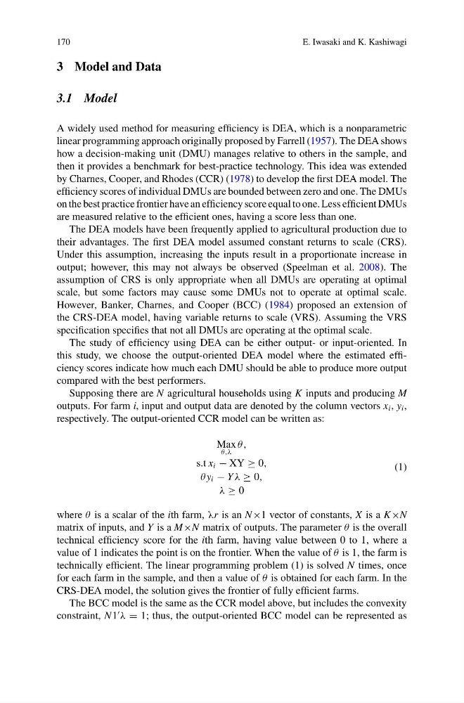
respectively. The output-oriented CCR model can be written as:
Max
θ,λ
θ,
s.t x i − XY ≥ 0,
θ y i − Y λ ≥ 0,
λ ≥ 0
(1)
where θ is a scalar of the ith farm, λr is an N×1 vector of constants, X is a K×N
matrix of inputs, and Y is a M×N matrix of outputs. The parameter θ is the overall
technical efficiency score for the ith farm, having value between 0 to 1, where a
value of 1 indicates the point is on the frontier. When the value of θ is 1, the farm is
technically efficient. The linear programming problem (1) is solved N times, once
for each farm in the sample, and then a value of θ is obtained for each farm. In the
CRS-DEA model, the solution gives the frontier of fully efficient farms.
The BCC model is the same as the CCR model above, but includes the convexity
constraint, N1
λ = 1; thus, the output-oriented BCC model can be represented as
E. Iwasaki and K. Kashiwagi
3 Model and Data
3.1 Model
A widely used method for measuring efficiency is DEA, which is a nonparametric
linear programming approach originally proposed by Farrell (1957). The DEA shows
how a decision-making unit (DMU) manages relative to others in the sample, and
then it provides a benchmark for best-practice technology. This idea was extended
by Charnes, Cooper, and Rhodes (CCR) (1978) to develop the first DEA model. The
efficiency scores of individual DMUs are bounded between zero and one. The DMUs
on the best practice frontier have an efficiency score equal to one. Less efficient DMUs
are measured relative to the efficient ones, having a score less than one.
The DEA models have been frequently applied to agricultural production due to
their advantages. The first DEA model assumed constant returns to scale (CRS).
Under this assumption, increasing the inputs result in a proportionate increase in
output; however, this may not always be observed (Speelman et al. 2008). The
assumption of CRS is only appropriate when all DMUs are operating at optimal
scale, but some factors may cause some DMUs not to operate at optimal scale.
However, Banker, Charnes, and Cooper (BCC) (1984) proposed an extension of
the CRS-DEA model, having variable returns to scale (VRS). Assuming the VRS
specification specifies that not all DMUs are operating at the optimal scale.
The study of efficiency using DEA can be either output- or input-oriented. In
this study, we choose the output-oriented DEA model where the estimated efficiency scores indicate how much each DMU should be able to produce more output
compared with the best performers.
Supposing there are N agricultural households using K inputs and producing M
outputs. For farm i, input and output data are denoted by the column vectors x i , y i ,
respectively. The output-oriented CCR model can be written as:
Max
θ,λ
θ,
s.t x i − XY ≥ 0,
θ y i − Y λ ≥ 0,
λ ≥ 0
(1)
where θ is a scalar of the ith farm, λr is an N×1 vector of constants, X is a K×N
matrix of inputs, and Y is a M×N matrix of outputs. The parameter θ is the overall
technical efficiency score for the ith farm, having value between 0 to 1, where a
value of 1 indicates the point is on the frontier. When the value of θ is 1, the farm is
technically efficient. The linear programming problem (1) is solved N times, once
for each farm in the sample, and then a value of θ is obtained for each farm. In the
CRS-DEA model, the solution gives the frontier of fully efficient farms.
The BCC model is the same as the CCR model above, but includes the convexity
constraint, N1
λ = 1; thus, the output-oriented BCC model can be represented as