

“Multiple Dividends with Climate Change Policies: Evidence …
109
The endowment of internationally mobile capital, owned by the domestic household, is given by K 0 and its remuneration is R
* . At the benchmark the proportion
of fixed capital owned by the domestic household with respect to mobile capital is
therefore 2/K 0 (in fact, this parameter can be unobservable and uncertain).
P 1 C 1 (1 + t 1 ) + P 2 C 2 = W L 0 + R
∗ K 0 + 1π 1 + 1π 2
(2)
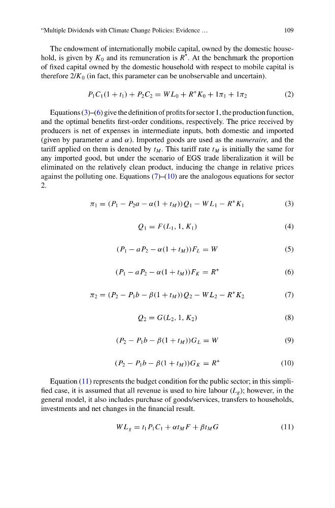
Equations (3)–(6) give the definition of profits for sector 1, the production function,
and the optimal benefits first-order conditions, respectively. The price received by
producers is net of expenses in intermediate inputs, both domestic and imported
(given by parameter a and α). Imported goods are used as the numeraire, and the
tariff applied on them is denoted by t M . This tariff rate t M is initially the same for
any imported good, but under the scenario of EGS trade liberalization it will be
eliminated on the relatively clean product, inducing the change in relative prices
against the polluting one. Equations (7)–(10) are the analogous equations for sector
2.
π 1 = (P 1 − P 2 a − α(1 + t M ))Q 1 − W L 1 − R
∗ K 1
(3)
Q 1 = F(L 1 , 1, K 1 )
(4)
(P 1 − a P 2 − α(1 + t M ))F L = W
(5)
(P 1 − a P 2 − α(1 + t M ))F K = R
∗
(6)
π 2 = (P 2 − P 1 b − β(1 + t M ))Q 2 − W L 2 − R
∗ K 2
(7)
Q 2 = G(L 2 , 1, K 2 )
(8)
(P 2 − P 1 b − β(1 + t M ))G L = W
(9)
(P 2 − P 1 b − β(1 + t M ))G K = R
∗
(10)
Equation (11) represents the budget condition for the public sector; in this simplified case, it is assumed that all revenue is used to hire labour (L g ); however, in the
general model, it also includes purchase of goods/services, transfers to households,
investments and net changes in the financial result.
W L g = t 1 P 1 C 1 + αt M F + βt M G
(11)
109
The endowment of internationally mobile capital, owned by the domestic household, is given by K 0 and its remuneration is R
* . At the benchmark the proportion
of fixed capital owned by the domestic household with respect to mobile capital is
therefore 2/K 0 (in fact, this parameter can be unobservable and uncertain).
P 1 C 1 (1 + t 1 ) + P 2 C 2 = W L 0 + R
∗ K 0 + 1π 1 + 1π 2
(2)
Equations (3)–(6) give the definition of profits for sector 1, the production function,
and the optimal benefits first-order conditions, respectively. The price received by
producers is net of expenses in intermediate inputs, both domestic and imported
(given by parameter a and α). Imported goods are used as the numeraire, and the
tariff applied on them is denoted by t M . This tariff rate t M is initially the same for
any imported good, but under the scenario of EGS trade liberalization it will be
eliminated on the relatively clean product, inducing the change in relative prices
against the polluting one. Equations (7)–(10) are the analogous equations for sector
2.
π 1 = (P 1 − P 2 a − α(1 + t M ))Q 1 − W L 1 − R
∗ K 1
(3)
Q 1 = F(L 1 , 1, K 1 )
(4)
(P 1 − a P 2 − α(1 + t M ))F L = W
(5)
(P 1 − a P 2 − α(1 + t M ))F K = R
∗
(6)
π 2 = (P 2 − P 1 b − β(1 + t M ))Q 2 − W L 2 − R
∗ K 2
(7)
Q 2 = G(L 2 , 1, K 2 )
(8)
(P 2 − P 1 b − β(1 + t M ))G L = W
(9)
(P 2 − P 1 b − β(1 + t M ))G K = R
∗
(10)
Equation (11) represents the budget condition for the public sector; in this simplified case, it is assumed that all revenue is used to hire labour (L g ); however, in the
general model, it also includes purchase of goods/services, transfers to households,
investments and net changes in the financial result.
W L g = t 1 P 1 C 1 + αt M F + βt M G
(11)