

110
M. P. Ramos and O. O. Chisari
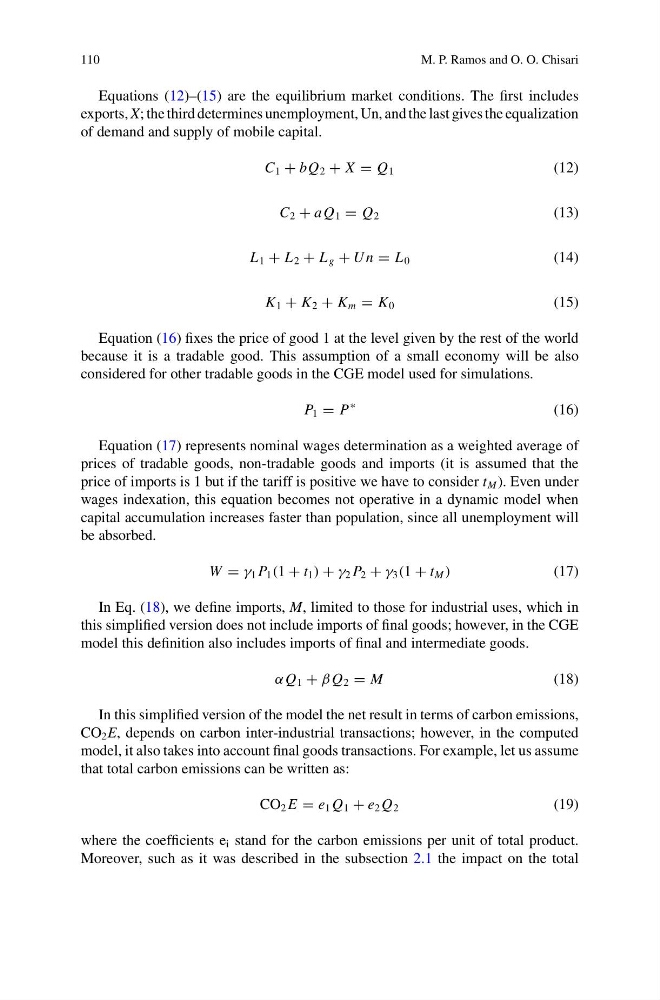
Equations (12)–(15) are the equilibrium market conditions. The first includes
exports, X; the third determines unemployment, Un, and the last gives the equalization
of demand and supply of mobile capital.
C 1 + bQ 2 + X = Q 1
(12)
C 2 + a Q 1 = Q 2
(13)
L 1 + L 2 + L g + U n = L 0
(14)
K 1 + K 2 + K m = K 0
(15)
Equation (16) fixes the price of good 1 at the level given by the rest of the world
because it is a tradable good. This assumption of a small economy will be also
considered for other tradable goods in the CGE model used for simulations.
P 1 = P
∗
(16)
Equation (17) represents nominal wages determination as a weighted average of
prices of tradable goods, non-tradable goods and imports (it is assumed that the
price of imports is 1 but if the tariff is positive we have to consider t M ). Even under
wages indexation, this equation becomes not operative in a dynamic model when
capital accumulation increases faster than population, since all unemployment will
be absorbed.
W = γ 1 P 1 (1 + t 1 ) + γ 2 P 2 + γ 3 (1 + t M )
(17)
In Eq. (18), we define imports, M, limited to those for industrial uses, which in
this simplified version does not include imports of final goods; however, in the CGE
model this definition also includes imports of final and intermediate goods.
α Q 1 + β Q 2 = M
(18)
In this simplified version of the model the net result in terms of carbon emissions,
CO 2 E, depends on carbon inter-industrial transactions; however, in the computed
model, it also takes into account final goods transactions. For example, let us assume
that total carbon emissions can be written as:
CO 2 E = e 1 Q 1 + e 2 Q 2
(19)
where the coefficients e i stand for the carbon emissions per unit of total product.
Moreover, such as it was described in the subsection 2.1 the impact on the total
M. P. Ramos and O. O. Chisari
Equations (12)–(15) are the equilibrium market conditions. The first includes
exports, X; the third determines unemployment, Un, and the last gives the equalization
of demand and supply of mobile capital.
C 1 + bQ 2 + X = Q 1
(12)
C 2 + a Q 1 = Q 2
(13)
L 1 + L 2 + L g + U n = L 0
(14)
K 1 + K 2 + K m = K 0
(15)
Equation (16) fixes the price of good 1 at the level given by the rest of the world
because it is a tradable good. This assumption of a small economy will be also
considered for other tradable goods in the CGE model used for simulations.
P 1 = P
∗
(16)
Equation (17) represents nominal wages determination as a weighted average of
prices of tradable goods, non-tradable goods and imports (it is assumed that the
price of imports is 1 but if the tariff is positive we have to consider t M ). Even under
wages indexation, this equation becomes not operative in a dynamic model when
capital accumulation increases faster than population, since all unemployment will
be absorbed.
W = γ 1 P 1 (1 + t 1 ) + γ 2 P 2 + γ 3 (1 + t M )
(17)
In Eq. (18), we define imports, M, limited to those for industrial uses, which in
this simplified version does not include imports of final goods; however, in the CGE
model this definition also includes imports of final and intermediate goods.
α Q 1 + β Q 2 = M
(18)
In this simplified version of the model the net result in terms of carbon emissions,
CO 2 E, depends on carbon inter-industrial transactions; however, in the computed
model, it also takes into account final goods transactions. For example, let us assume
that total carbon emissions can be written as:
CO 2 E = e 1 Q 1 + e 2 Q 2
(19)
where the coefficients e i stand for the carbon emissions per unit of total product.
Moreover, such as it was described in the subsection 2.1 the impact on the total