

Statistical Optimization of Ammonium Sulfamate and Urea-Based Fire …
121
the corresponding variation in two input process variables A and B as given below.
As per the new test run set, the RSM design layout UDQM experimental design
technique is used to vary one parameter at a time while keeping the other constant as
given in Table 6 and all the experiments are repeated three times and data represented
for the response variables (in Results and discussion) are the average value of those
three repeat test results in each case.
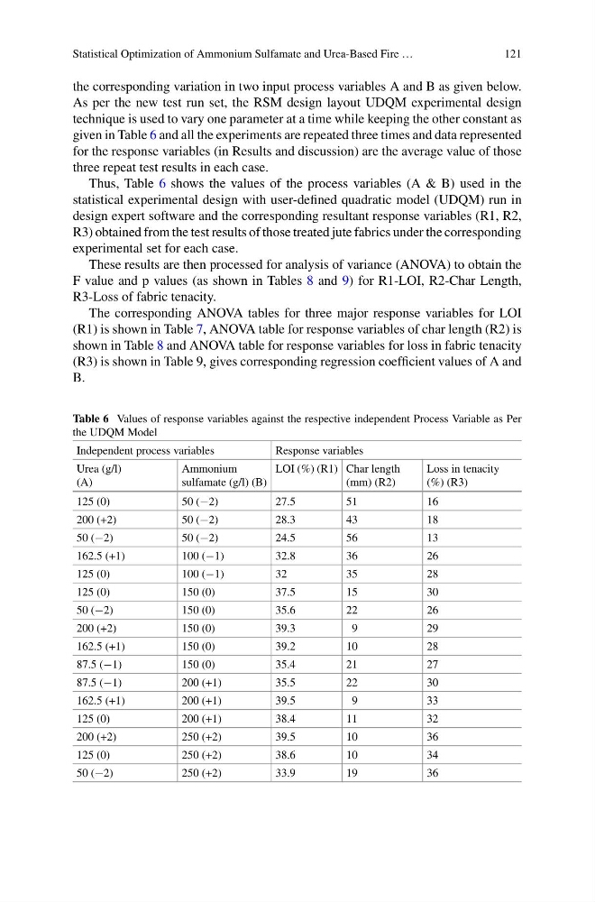
Thus, Table 6 shows the values of the process variables (A & B) used in the
statistical experimental design with user-defined quadratic model (UDQM) run in
design expert software and the corresponding resultant response variables (R1, R2,
R3) obtained from the test results of those treated jute fabrics under the corresponding
experimental set for each case.
These results are then processed for analysis of variance (ANOVA) to obtain the
F value and p values (as shown in Tables 8 and 9) for R1-LOI, R2-Char Length,
R3-Loss of fabric tenacity.
The corresponding ANOVA tables for three major response variables for LOI
(R1) is shown in Table 7, ANOVA table for response variables of char length (R2) is
shown in Table 8 and ANOVA table for response variables for loss in fabric tenacity
(R3) is shown in Table 9, gives corresponding regression coefficient values of A and
B.
Table 6 Values of response variables against the respective independent Process Variable as Per
the UDQM Model
Independent process variables
Response variables
Urea (g/l)
(A)
Ammonium
sulfamate (g/l) (B)
LOI (%) (R1) Char length
(mm) (R2)
Loss in tenacity
(%) (R3)
125 (0)
50 (−2)
27.5
51
16
200 (+2)
50 (−2)
28.3
43
18
50 (−2)
50 (−2)
24.5
56
13
162.5 (+1)
100 (−1)
32.8
36
26
125 (0)
100 (−1)
32
35
28
125 (0)
150 (0)
37.5
15
30
50 (−2)
150 (0)
35.6
22
26
200 (+2)
150 (0)
39.3
9
29
162.5 (+1)
150 (0)
39.2
10
28
87.5 (−1)
150 (0)
35.4
21
27
87.5 (−1)
200 (+1)
35.5
22
30
162.5 (+1)
200 (+1)
39.5
9
33
125 (0)
200 (+1)
38.4
11
32
200 (+2)
250 (+2)
39.5
10
36
125 (0)
250 (+2)
38.6
10
34
50 (−2)
250 (+2)
33.9
19
36
121
the corresponding variation in two input process variables A and B as given below.
As per the new test run set, the RSM design layout UDQM experimental design
technique is used to vary one parameter at a time while keeping the other constant as
given in Table 6 and all the experiments are repeated three times and data represented
for the response variables (in Results and discussion) are the average value of those
three repeat test results in each case.
Thus, Table 6 shows the values of the process variables (A & B) used in the
statistical experimental design with user-defined quadratic model (UDQM) run in
design expert software and the corresponding resultant response variables (R1, R2,
R3) obtained from the test results of those treated jute fabrics under the corresponding
experimental set for each case.
These results are then processed for analysis of variance (ANOVA) to obtain the
F value and p values (as shown in Tables 8 and 9) for R1-LOI, R2-Char Length,
R3-Loss of fabric tenacity.
The corresponding ANOVA tables for three major response variables for LOI
(R1) is shown in Table 7, ANOVA table for response variables of char length (R2) is
shown in Table 8 and ANOVA table for response variables for loss in fabric tenacity
(R3) is shown in Table 9, gives corresponding regression coefficient values of A and
B.
Table 6 Values of response variables against the respective independent Process Variable as Per
the UDQM Model
Independent process variables
Response variables
Urea (g/l)
(A)
Ammonium
sulfamate (g/l) (B)
LOI (%) (R1) Char length
(mm) (R2)
Loss in tenacity
(%) (R3)
125 (0)
50 (−2)
27.5
51
16
200 (+2)
50 (−2)
28.3
43
18
50 (−2)
50 (−2)
24.5
56
13
162.5 (+1)
100 (−1)
32.8
36
26
125 (0)
100 (−1)
32
35
28
125 (0)
150 (0)
37.5
15
30
50 (−2)
150 (0)
35.6
22
26
200 (+2)
150 (0)
39.3
9
29
162.5 (+1)
150 (0)
39.2
10
28
87.5 (−1)
150 (0)
35.4
21
27
87.5 (−1)
200 (+1)
35.5
22
30
162.5 (+1)
200 (+1)
39.5
9
33
125 (0)
200 (+1)
38.4
11
32
200 (+2)
250 (+2)
39.5
10
36
125 (0)
250 (+2)
38.6
10
34
50 (−2)
250 (+2)
33.9
19
36