

86
5 Higher Order Moment Robust Filtering …
˙
V (t) = ˙ ˜
S
T (t, p)F ˜
S(t, p) + ˜
S
T
(t, p)F ˙ ˜
S(t, p)
= ˜
S
T
(t, p)
˜
A
T F + F ˜
A
S(t, p) + ˜
S
T
(t, p)F ˜
Bω N p (t) + ω
T
N p (t) ˜
B
T F ˜
S(t, p)
= η
T
(t)
F ˜
A + ˜
A
T F F ˜
B
˜
B
T F
0
η(t),
(5.47)
where η(t)
T
=
˜
S
T
(t, p) ω
T
N p (t)
.
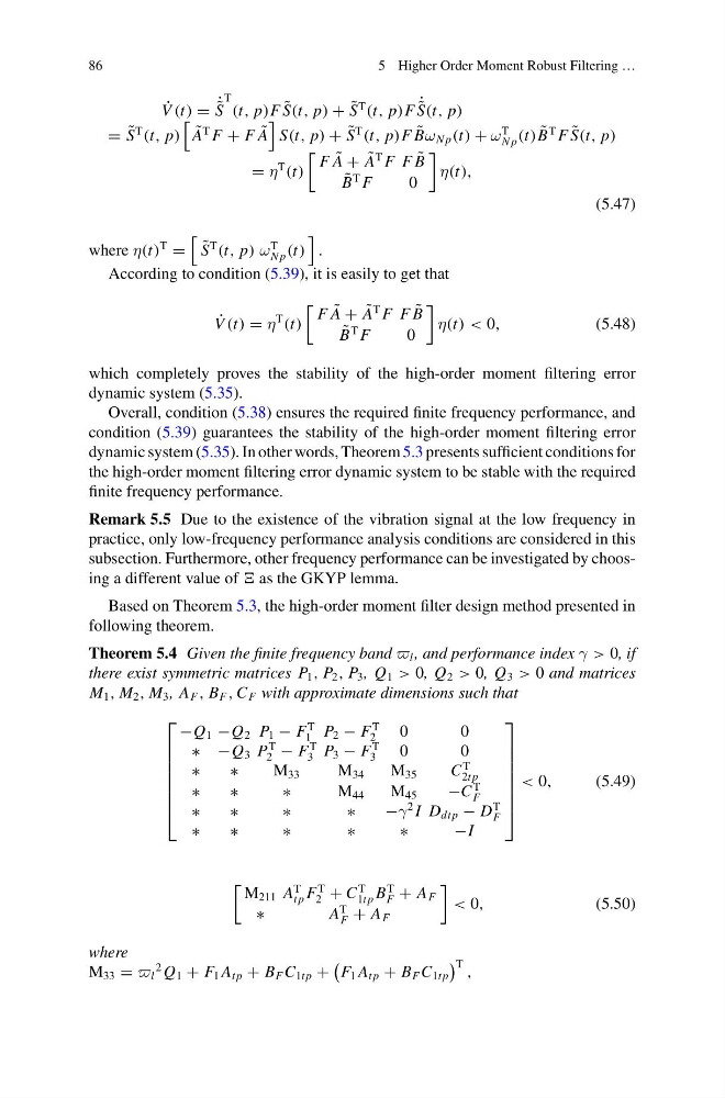
According to condition (5.39), it is easily to get that
˙
V (t) = η
T
(t)
F ˜
A + ˜
A
T F F ˜
B
˜
B
T F
0
η(t) < 0,
(5.48)
which completely proves the stability of the high-order moment filtering error
dynamic system (5.35).
Overall, condition (5.38) ensures the required finite frequency performance, and
condition (5.39) guarantees the stability of the high-order moment filtering error
dynamic system (5.35). In other words, Theorem 5.3 presents sufficient conditions for
the high-order moment filtering error dynamic system to be stable with the required
finite frequency performance.
Remark 5.5 Due to the existence of the vibration signal at the low frequency in
practice, only low-frequency performance analysis conditions are considered in this
subsection. Furthermore, other frequency performance can be investigated by choosing a different value of as the GKYP lemma.
Based on Theorem 5.3, the high-order moment filter design method presented in
following theorem.
Theorem 5.4 Given the finite frequency band l , and performance index γ > 0, if
there exist symmetric matrices P 1 , P 2 , P 3 , Q 1 > 0, Q 2 > 0, Q 3 > 0 and matrices
M 1 , M 2 , M 3 , A F , B F , C F with approximate dimensions such that
⎡
⎢
⎢
⎢
⎢
⎢
⎢
⎣
−Q 1 −Q 2 P 1 − F
T
1 P 2 − F
T
2
0
0
∗ −Q 3 P
T
2 − F
T
3 P 3 − F
T
3
0
0
∗
∗
M 33
M 34
M 35
C
T
2tp
∗
∗
∗
M 44
M 45
−C
T
F
∗
∗
∗
∗
−γ
2 I D dt p − D
T
F
∗
∗
∗
∗
∗
−I
⎤
⎥
⎥
⎥
⎥
⎥
⎥
⎦
< 0,
(5.49)
M 211 A
T
tp F
T
2 + C
T
1tp B
T
F + A F
∗
A
T
F + A F
< 0,
(5.50)
where
M 33 = l
2 Q 1 + F 1 A tp + B F C 1tp +
F 1 A tp + B F C 1tp
T ,
5 Higher Order Moment Robust Filtering …
˙
V (t) = ˙ ˜
S
T (t, p)F ˜
S(t, p) + ˜
S
T
(t, p)F ˙ ˜
S(t, p)
= ˜
S
T
(t, p)
˜
A
T F + F ˜
A
S(t, p) + ˜
S
T
(t, p)F ˜
Bω N p (t) + ω
T
N p (t) ˜
B
T F ˜
S(t, p)
= η
T
(t)
F ˜
A + ˜
A
T F F ˜
B
˜
B
T F
0
η(t),
(5.47)
where η(t)
T
=
˜
S
T
(t, p) ω
T
N p (t)
.
According to condition (5.39), it is easily to get that
˙
V (t) = η
T
(t)
F ˜
A + ˜
A
T F F ˜
B
˜
B
T F
0
η(t) < 0,
(5.48)
which completely proves the stability of the high-order moment filtering error
dynamic system (5.35).
Overall, condition (5.38) ensures the required finite frequency performance, and
condition (5.39) guarantees the stability of the high-order moment filtering error
dynamic system (5.35). In other words, Theorem 5.3 presents sufficient conditions for
the high-order moment filtering error dynamic system to be stable with the required
finite frequency performance.
Remark 5.5 Due to the existence of the vibration signal at the low frequency in
practice, only low-frequency performance analysis conditions are considered in this
subsection. Furthermore, other frequency performance can be investigated by choosing a different value of as the GKYP lemma.
Based on Theorem 5.3, the high-order moment filter design method presented in
following theorem.
Theorem 5.4 Given the finite frequency band l , and performance index γ > 0, if
there exist symmetric matrices P 1 , P 2 , P 3 , Q 1 > 0, Q 2 > 0, Q 3 > 0 and matrices
M 1 , M 2 , M 3 , A F , B F , C F with approximate dimensions such that
⎡
⎢
⎢
⎢
⎢
⎢
⎢
⎣
−Q 1 −Q 2 P 1 − F
T
1 P 2 − F
T
2
0
0
∗ −Q 3 P
T
2 − F
T
3 P 3 − F
T
3
0
0
∗
∗
M 33
M 34
M 35
C
T
2tp
∗
∗
∗
M 44
M 45
−C
T
F
∗
∗
∗
∗
−γ
2 I D dt p − D
T
F
∗
∗
∗
∗
∗
−I
⎤
⎥
⎥
⎥
⎥
⎥
⎥
⎦
< 0,
(5.49)
M 211 A
T
tp F
T
2 + C
T
1tp B
T
F + A F
∗
A
T
F + A F
< 0,
(5.50)
where
M 33 = l
2 Q 1 + F 1 A tp + B F C 1tp +
F 1 A tp + B F C 1tp
T ,