

5.2 High-Order Moment Filtering for Multi-model Jumping …
87
M 34 =
2
l Q 2 + A F +
F 2 A tp + B F C 1tp
T ,
M 44 = l
2 Q 3 + A F + A F
T
,
M 35 = F 1 B dt p + B F D dt p ,
M 45 = F 2 B dt p + B F D dt p ,
M 211 = A
T
tp F
T
1 + F 1 A tp + C
T
1tp B
T
F + B F C 1tp .
Then a filter of form (5.34) must satisfy the mean stability of the high-order moment
filtering error dynamic system (5.35) with the required finite frequency performance
γ . The filter realization is given by
A f = F
−1
2 A F , B f = F
−1
2 B F , C f = C F , D f = D F .
(5.51)
Proof Based on Theorem 3.1, conditions (5.38) and (5.39) ensure that filtering system (5.35) is stable with the required finite frequency performance γ. Choosing the
structures of P, Q and F as
P =
P 1 P 2
∗ P 3
, Q =
Q 1 Q 2
∗ Q 3
, F =
F 1 F 3
F 2 F 3
Letting
A F = F 2 A f , B F = F 2 B f , C F = C f , D F = D f ,
after changes in variables and an equivalent transformation, it follows that inequality (5.49) is equivalent to inequality (5.38), and inequality (5.50) is equivalent to
inequality (5.39). It completes the proof.
5.3 Numeral Examples
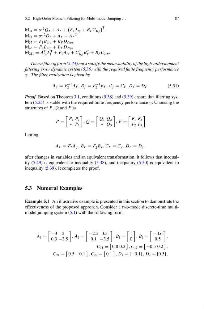
Example 5.1 An illustrative example is presented in this section to demonstrate the
effectiveness of the proposed approach. Consider a two-mode discrete-time multimodel jumping system (5.1) with the following form:
A 1 =
−3 2
0.3 −2.5
, A 2 =
−2.5 0.5
0.1 −3.5
, B 1 =
1
0
, B 2 =
−0.6
0.5
,
C 11 =
0.8 0.3
, C 12 =
−0.5 0.2
,
C 21 =
0.5 −0.1
, C 22 =
0 1
, D 1 = [−0.1] , D 2 = [0.5] .
87
M 34 =
2
l Q 2 + A F +
F 2 A tp + B F C 1tp
T ,
M 44 = l
2 Q 3 + A F + A F
T
,
M 35 = F 1 B dt p + B F D dt p ,
M 45 = F 2 B dt p + B F D dt p ,
M 211 = A
T
tp F
T
1 + F 1 A tp + C
T
1tp B
T
F + B F C 1tp .
Then a filter of form (5.34) must satisfy the mean stability of the high-order moment
filtering error dynamic system (5.35) with the required finite frequency performance
γ . The filter realization is given by
A f = F
−1
2 A F , B f = F
−1
2 B F , C f = C F , D f = D F .
(5.51)
Proof Based on Theorem 3.1, conditions (5.38) and (5.39) ensure that filtering system (5.35) is stable with the required finite frequency performance γ. Choosing the
structures of P, Q and F as
P =
P 1 P 2
∗ P 3
, Q =
Q 1 Q 2
∗ Q 3
, F =
F 1 F 3
F 2 F 3
Letting
A F = F 2 A f , B F = F 2 B f , C F = C f , D F = D f ,
after changes in variables and an equivalent transformation, it follows that inequality (5.49) is equivalent to inequality (5.38), and inequality (5.50) is equivalent to
inequality (5.39). It completes the proof.
5.3 Numeral Examples
Example 5.1 An illustrative example is presented in this section to demonstrate the
effectiveness of the proposed approach. Consider a two-mode discrete-time multimodel jumping system (5.1) with the following form:
A 1 =
−3 2
0.3 −2.5
, A 2 =
−2.5 0.5
0.1 −3.5
, B 1 =
1
0
, B 2 =
−0.6
0.5
,
C 11 =
0.8 0.3
, C 12 =
−0.5 0.2
,
C 21 =
0.5 −0.1
, C 22 =
0 1
, D 1 = [−0.1] , D 2 = [0.5] .