

5.2 High-Order Moment Filtering for Multi-model Jumping …
85
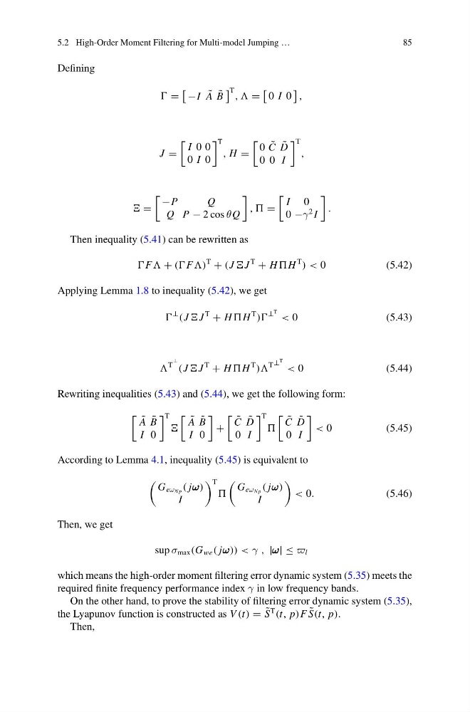
Defining
=
−I ˜
A ˜
B
T , , =
0 I 0
,
J =
I 0 0
0 I 0
T
, H =
0 ˜
C ˜
D
0 0 I
T
,
=
−P
Q
Q P − 2 cos θ Q
, , =
I 0
0 −γ
2 I
.
Then inequality (5.41) can be rewritten as
F + (( F)
T
+ (J J
T
+ H H
T
) < 0
(5.42)
Applying Lemma 1.8 to inequality (5.42), we get
⊥
(J J
T
+ H H
T
))
⊥
T < 0
(5.43)
T
⊥ (J J
T
+ H H
T
))
T ⊥
T < 0
(5.44)
Rewriting inequalities (5.43) and (5.44), we get the following form:
˜
A ˜
B
I 0
T
˜
A ˜
B
I 0
+
˜
C ˜
D
0 I
T
˜
C ˜
D
0 I
< 0
(5.45)
According to Lemma 4.1, inequality (5.45) is equivalent to
G eω N p ( jω ω ω)
I
T
G eω N p ( jω ω ω)
I
< 0.
(5.46)
Then, we get
sup σ max (G we ( jω ω ω)) < γ , |ω ω ω| ≤ l
which means the high-order moment filtering error dynamic system (5.35) meets the
required finite frequency performance index γ in low frequency bands.
On the other hand, to prove the stability of filtering error dynamic system (5.35),
the Lyapunov function is constructed as V (t) = ˜
S
T
(t, p)F ˜
S(t, p).
Then,
85
Defining
=
−I ˜
A ˜
B
T , , =
0 I 0
,
J =
I 0 0
0 I 0
T
, H =
0 ˜
C ˜
D
0 0 I
T
,
=
−P
Q
Q P − 2 cos θ Q
, , =
I 0
0 −γ
2 I
.
Then inequality (5.41) can be rewritten as
F + (( F)
T
+ (J J
T
+ H H
T
) < 0
(5.42)
Applying Lemma 1.8 to inequality (5.42), we get
⊥
(J J
T
+ H H
T
))
⊥
T < 0
(5.43)
T
⊥ (J J
T
+ H H
T
))
T ⊥
T < 0
(5.44)
Rewriting inequalities (5.43) and (5.44), we get the following form:
˜
A ˜
B
I 0
T
˜
A ˜
B
I 0
+
˜
C ˜
D
0 I
T
˜
C ˜
D
0 I
< 0
(5.45)
According to Lemma 4.1, inequality (5.45) is equivalent to
G eω N p ( jω ω ω)
I
T
G eω N p ( jω ω ω)
I
< 0.
(5.46)
Then, we get
sup σ max (G we ( jω ω ω)) < γ , |ω ω ω| ≤ l
which means the high-order moment filtering error dynamic system (5.35) meets the
required finite frequency performance index γ in low frequency bands.
On the other hand, to prove the stability of filtering error dynamic system (5.35),
the Lyapunov function is constructed as V (t) = ˜
S
T
(t, p)F ˜
S(t, p).
Then,