

84
5 Higher Order Moment Robust Filtering …
l , 1 , 2 , and h are the given finite frequency ranges for low-frequency range,
middle-frequency range, and high-frequency range,respectively. Moreover, the c
is given as c = ( 1 + 2 )/2.
Remark 5.4 The matrix in the GKYP lemma describes the finite frequency performance of the system. In this chapter, we consider the H ∞ performance of the
filtering error dynamic system (5.35). Therefore, we take =
I 0
0 −γ
2 I
.
5.2.2 High-Order Moment Finite Frequency Filter Design
Assuming the filter parameters are known, the following theorem provides sufficient
conditions under which the high-order moment filtering error dynamic system (5.35)
is stable with a prescribed finite frequency disturbance rejection level.
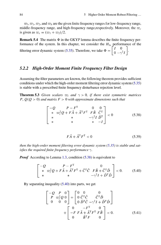
Theorem 5.3 Given scalars l and γ > 0, if there exist symmetric matrices
P, Q(Q > 0) and matrix F > 0 with approximate dimensions such that
⎡
⎢
⎢
⎣
−Q
P− F
T
0
0
∗
2
l Q + F ˜
A + ˜
A
T F
T F ˜
B ˜
C
T
∗
∗
− γ
2 I ˜
D
T
∗
∗
∗ − I
⎤
⎥
⎥
⎦ < 0
(5.38)
F ˜
A + ˜
A
T F
T
< 0
(5.39)
then the high-order moment filtering error dynamic system (5.35) is stable and satisfies the required finite frequency performance γ.
Proof According to Lemma 1.3, condition (5.38) is equivalent to
⎡
⎣
−Q
P− F
T
0
∗
2
l Q + F ˜
A + ˜
A
T F
T
+ ˜
C
T ˜
C F ˜
B + ˜
C
T ˜
D
∗
∗
− γ
2 I + ˜
D
T ˜
D
⎤
⎦ < 0.
(5.40)
By separating inequality (5.40) into parts, we get
⎡
⎣
−Q P 0
P
2
l Q 0
0
0 0
⎤
⎦ +
⎡
⎣
0 0
0
0 ˜
C
T ˜
C
˜
C
T ˜
D
0 ˜
D
T ˜
C −γ
2 I + ˜
D
T ˜
D
⎤
⎦
+
⎡
⎣
0
−F
T
0
−F F ˜
A + ˜
A
T F
T F ˜
B
0
˜
B
T F
0
⎤
⎦ < 0.
(5.41)
5 Higher Order Moment Robust Filtering …
l , 1 , 2 , and h are the given finite frequency ranges for low-frequency range,
middle-frequency range, and high-frequency range,respectively. Moreover, the c
is given as c = ( 1 + 2 )/2.
Remark 5.4 The matrix in the GKYP lemma describes the finite frequency performance of the system. In this chapter, we consider the H ∞ performance of the
filtering error dynamic system (5.35). Therefore, we take =
I 0
0 −γ
2 I
.
5.2.2 High-Order Moment Finite Frequency Filter Design
Assuming the filter parameters are known, the following theorem provides sufficient
conditions under which the high-order moment filtering error dynamic system (5.35)
is stable with a prescribed finite frequency disturbance rejection level.
Theorem 5.3 Given scalars l and γ > 0, if there exist symmetric matrices
P, Q(Q > 0) and matrix F > 0 with approximate dimensions such that
⎡
⎢
⎢
⎣
−Q
P− F
T
0
0
∗
2
l Q + F ˜
A + ˜
A
T F
T F ˜
B ˜
C
T
∗
∗
− γ
2 I ˜
D
T
∗
∗
∗ − I
⎤
⎥
⎥
⎦ < 0
(5.38)
F ˜
A + ˜
A
T F
T
< 0
(5.39)
then the high-order moment filtering error dynamic system (5.35) is stable and satisfies the required finite frequency performance γ.
Proof According to Lemma 1.3, condition (5.38) is equivalent to
⎡
⎣
−Q
P− F
T
0
∗
2
l Q + F ˜
A + ˜
A
T F
T
+ ˜
C
T ˜
C F ˜
B + ˜
C
T ˜
D
∗
∗
− γ
2 I + ˜
D
T ˜
D
⎤
⎦ < 0.
(5.40)
By separating inequality (5.40) into parts, we get
⎡
⎣
−Q P 0
P
2
l Q 0
0
0 0
⎤
⎦ +
⎡
⎣
0 0
0
0 ˜
C
T ˜
C
˜
C
T ˜
D
0 ˜
D
T ˜
C −γ
2 I + ˜
D
T ˜
D
⎤
⎦
+
⎡
⎣
0
−F
T
0
−F F ˜
A + ˜
A
T F
T F ˜
B
0
˜
B
T F
0
⎤
⎦ < 0.
(5.41)