

5.2 High-Order Moment Filtering for Multi-model Jumping …
83
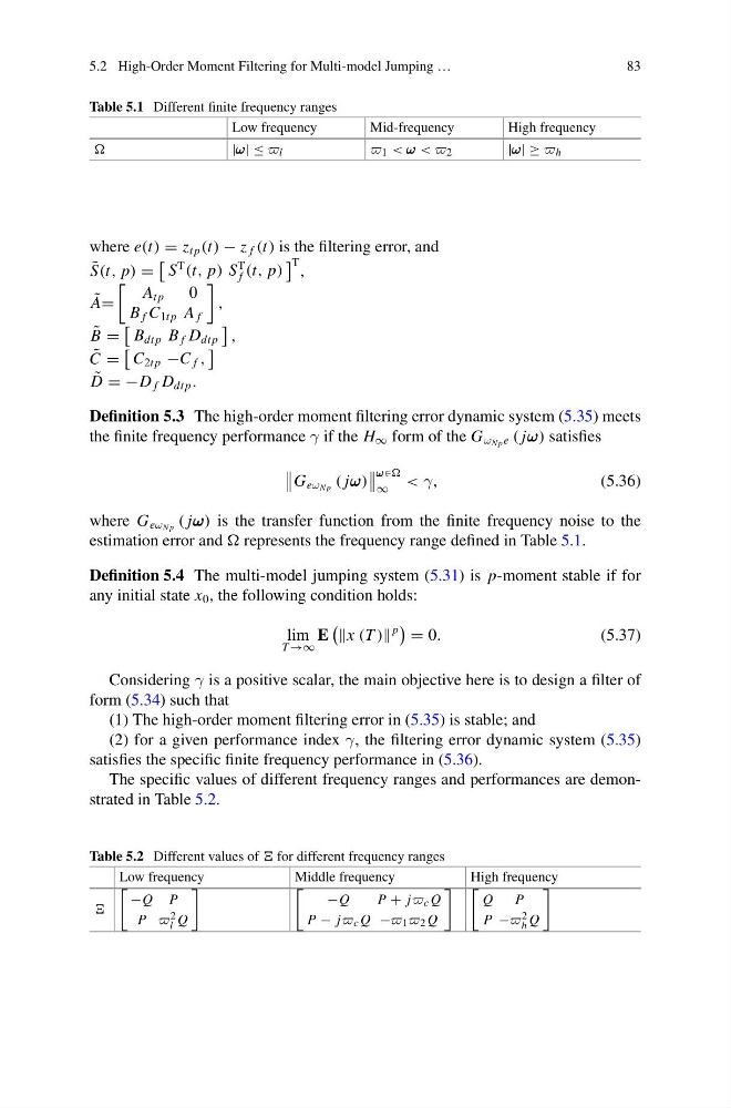
Table 5.1 Different finite frequency ranges
Low frequency
Mid-frequency
High frequency
|ω ω ω| ≤ l
1 < ω ω ω < 2
|ω ω ω| ≥ h
where e(t) = z tp (t) − z f (t) is the filtering error, and
˜
S(t, p) =
S
T
(t, p) S
T
f (t, p)
T ,
˜
A=
A tp
0
B f C 1tp A f
,
˜
B =
B dt p B f D dt p
,
˜
C =
C 2tp −C f ,
˜
D = −D f D dt p .
Definition 5.3 The high-order moment filtering error dynamic system (5.35) meets
the finite frequency performance γ if the H ∞ form of the G ω N p e ( jω ω ω) satisfies
G eω N p ( jω ω ω)
ω ω ω∈
∞
< γ,
(5.36)
where G eω N p ( jω ω ω) is the transfer function from the finite frequency noise to the
estimation error and represents the frequency range defined in Table 5.1.
Definition 5.4 The multi-model jumping system (5.31) is p-moment stable if for
any initial state x 0 , the following condition holds:
lim
T →∞
E
x (T )
p
= 0.
(5.37)
Considering γ is a positive scalar, the main objective here is to design a filter of
form (5.34) such that
(1) The high-order moment filtering error in (5.35) is stable; and
(2) for a given performance index γ, the filtering error dynamic system (5.35)
satisfies the specific finite frequency performance in (5.36).
The specific values of different frequency ranges and performances are demonstrated in Table 5.2.
Table 5.2 Different values of for different frequency ranges
Low frequency
Middle frequency
High frequency
−Q P
P 2
l Q
−Q
P+ j c Q
P − j c Q − 1 2 Q
Q
P
P − 2
h Q
83
Table 5.1 Different finite frequency ranges
Low frequency
Mid-frequency
High frequency
|ω ω ω| ≤ l
1 < ω ω ω < 2
|ω ω ω| ≥ h
where e(t) = z tp (t) − z f (t) is the filtering error, and
˜
S(t, p) =
S
T
(t, p) S
T
f (t, p)
T ,
˜
A=
A tp
0
B f C 1tp A f
,
˜
B =
B dt p B f D dt p
,
˜
C =
C 2tp −C f ,
˜
D = −D f D dt p .
Definition 5.3 The high-order moment filtering error dynamic system (5.35) meets
the finite frequency performance γ if the H ∞ form of the G ω N p e ( jω ω ω) satisfies
G eω N p ( jω ω ω)
ω ω ω∈
∞
< γ,
(5.36)
where G eω N p ( jω ω ω) is the transfer function from the finite frequency noise to the
estimation error and represents the frequency range defined in Table 5.1.
Definition 5.4 The multi-model jumping system (5.31) is p-moment stable if for
any initial state x 0 , the following condition holds:
lim
T →∞
E
x (T )
p
= 0.
(5.37)
Considering γ is a positive scalar, the main objective here is to design a filter of
form (5.34) such that
(1) The high-order moment filtering error in (5.35) is stable; and
(2) for a given performance index γ, the filtering error dynamic system (5.35)
satisfies the specific finite frequency performance in (5.36).
The specific values of different frequency ranges and performances are demonstrated in Table 5.2.
Table 5.2 Different values of for different frequency ranges
Low frequency
Middle frequency
High frequency
−Q P
P 2
l Q
−Q
P+ j c Q
P − j c Q − 1 2 Q
Q
P
P − 2
h Q