

3.3 Numeral Examples
45
0
1
2
3
4
5
6
7
8
9
10
0
0.5
1
1.5
2
2.5
3
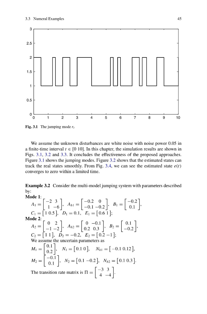
Fig. 3.1 The jumping mode r t
We assume the unknown disturbances are white noise with noise power 0.05 in
a finite-time interval t ∈ [0 10]. In this chapter, the simulation results are shown in
Figs. 3.1, 3.2 and 3.3. It concludes the effectiveness of the proposed approaches.
Figure 3.1 shows the jumping modes. Figure 3.2 shows that the estimated states can
track the real states smoothly. From Fig. 3.4, we can see the estimated state e(t)
converges to zero within a limited time.
Example 3.2 Consider the multi-model jumping system with parameters described
by:
Mode 1:
A 1 =
−2 3
1 −6
, A h1 =
−0.2 0
−0.1 −0.2
, B 1 =
−0.2
0.1
,
C 1 =
1 0.5
, D 1 = 0.1, E 1 =
0.6 1
;
Mode 2:
A 2 =
0 2
−1 −2
, A h2 =
0 −0.1
0.2 0.3
, B 2 =
0.1
−0.2
,
C 2 =
1 1
, D 2 = −0.2, E 2 =
0.2 −1
;
We assume the uncertain parameters as
M 1 =
0.1
0.2
, N 1 =
0.1 0
, N h1 =
−0.1 0.12
,
M 2 =
−0.1
0.1
, N 2 =
0.1 −0.2
, N h2 =
0.1 0.3
.
The transition rate matrix is =
−3 3
4 −4
.
45
0
1
2
3
4
5
6
7
8
9
10
0
0.5
1
1.5
2
2.5
3
Fig. 3.1 The jumping mode r t
We assume the unknown disturbances are white noise with noise power 0.05 in
a finite-time interval t ∈ [0 10]. In this chapter, the simulation results are shown in
Figs. 3.1, 3.2 and 3.3. It concludes the effectiveness of the proposed approaches.
Figure 3.1 shows the jumping modes. Figure 3.2 shows that the estimated states can
track the real states smoothly. From Fig. 3.4, we can see the estimated state e(t)
converges to zero within a limited time.
Example 3.2 Consider the multi-model jumping system with parameters described
by:
Mode 1:
A 1 =
−2 3
1 −6
, A h1 =
−0.2 0
−0.1 −0.2
, B 1 =
−0.2
0.1
,
C 1 =
1 0.5
, D 1 = 0.1, E 1 =
0.6 1
;
Mode 2:
A 2 =
0 2
−1 −2
, A h2 =
0 −0.1
0.2 0.3
, B 2 =
0.1
−0.2
,
C 2 =
1 1
, D 2 = −0.2, E 2 =
0.2 −1
;
We assume the uncertain parameters as
M 1 =
0.1
0.2
, N 1 =
0.1 0
, N h1 =
−0.1 0.12
,
M 2 =
−0.1
0.1
, N 2 =
0.1 −0.2
, N h2 =
0.1 0.3
.
The transition rate matrix is =
−3 3
4 −4
.