

2.1 Robust H ∞ Filtering for Multi-model Jumping Systems
19
words, we reduce γ
2 to the minimum possible value such that LMI (2.8) is satisfied,
i,e.,
min P i ,X i ,Y i ,C Fi ,D Fi ,Q,λ i , ˜
γ ˜
γ,
s.t. LMI (2.8) with ˜
γ = γ
2
.
(2.18)
Remark 2.1 The solutions of Theorems 2.1 and 2.2 can be obtained by solving an
optimization problem. By using the Matlab LMI Toolbox, it is straightforward to
check the feasibility of LMI (2.8). The effectiveness of the designed result will be
shown in (2.3) by using a numerical example.
2.2 Unbiased H ∞ Filtering for Multi-model Jumping
System
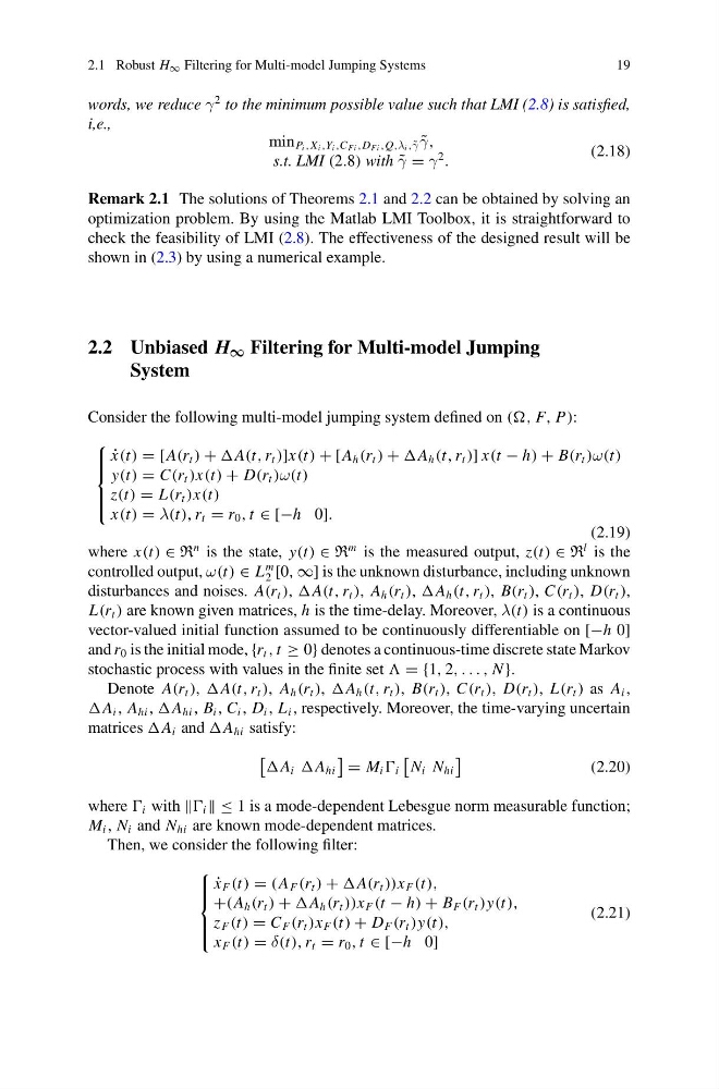
Consider the following multi-model jumping system defined on ((, F, P):
⎧
⎪ ⎪ ⎨
⎪ ⎪ ⎩
˙
x(t) = [A(r t ) + A(t, r t )]x(t) + [A h (r t ) + A h (t, r t )] x(t − h) + B(r t )ω(t)
y(t) = C(r t )x(t) + D(r t )ω(t)
z(t) = L(r t )x(t)
x(t) = λ(t), r t = r 0 , t ∈ [−h 0].
(2.19)
where x(t) ∈ R
n is the state, y(t) ∈ R
m is the measured output, z(t) ∈ R
l is the
controlled output, ω(t) ∈ L
m
2 [0, ∞] is the unknown disturbance, including unknown
disturbances and noises. A(r t ), A(t, r t ), A h (r t ), A h (t, r t ), B(r t ), C(r t ), D(r t ),
L(r t ) are known given matrices, h is the time-delay. Moreover, λ(t) is a continuous
vector-valued initial function assumed to be continuously differentiable on [−h 0]
and r 0 is the initial mode, {r t , t ≥ 0} denotes a continuous-time discrete state Markov
stochastic process with values in the finite set = {1, 2, . . . , N }.
Denote A(r t ), A(t, r t ), A h (r t ), A h (t, r t ), B(r t ), C(r t ), D(r t ), L(r t ) as A i ,
A i , A hi , A hi , B i , C i , D i , L i , respectively. Moreover, the time-varying uncertain
matrices A i and A hi satisfy:
A i A hi
= M i i
N i N hi
(2.20)
where i with i ≤ 1 is a mode-dependent Lebesgue norm measurable function;
M i , N i and N hi are known mode-dependent matrices.
Then, we consider the following filter:
⎧
⎪ ⎪ ⎨
⎪ ⎪ ⎩
˙
x F (t) = (A F (r t ) + A(r t ))x F (t),
+(A h (r t ) + A h (r t ))x F (t − h) + B F (r t )y(t),
z F (t) = C F (r t )x F (t) + D F (r t )y(t),
x F (t) = δ(t), r t = r 0 , t ∈ [−h 0]
(2.21)
19
words, we reduce γ
2 to the minimum possible value such that LMI (2.8) is satisfied,
i,e.,
min P i ,X i ,Y i ,C Fi ,D Fi ,Q,λ i , ˜
γ ˜
γ,
s.t. LMI (2.8) with ˜
γ = γ
2
.
(2.18)
Remark 2.1 The solutions of Theorems 2.1 and 2.2 can be obtained by solving an
optimization problem. By using the Matlab LMI Toolbox, it is straightforward to
check the feasibility of LMI (2.8). The effectiveness of the designed result will be
shown in (2.3) by using a numerical example.
2.2 Unbiased H ∞ Filtering for Multi-model Jumping
System
Consider the following multi-model jumping system defined on ((, F, P):
⎧
⎪ ⎪ ⎨
⎪ ⎪ ⎩
˙
x(t) = [A(r t ) + A(t, r t )]x(t) + [A h (r t ) + A h (t, r t )] x(t − h) + B(r t )ω(t)
y(t) = C(r t )x(t) + D(r t )ω(t)
z(t) = L(r t )x(t)
x(t) = λ(t), r t = r 0 , t ∈ [−h 0].
(2.19)
where x(t) ∈ R
n is the state, y(t) ∈ R
m is the measured output, z(t) ∈ R
l is the
controlled output, ω(t) ∈ L
m
2 [0, ∞] is the unknown disturbance, including unknown
disturbances and noises. A(r t ), A(t, r t ), A h (r t ), A h (t, r t ), B(r t ), C(r t ), D(r t ),
L(r t ) are known given matrices, h is the time-delay. Moreover, λ(t) is a continuous
vector-valued initial function assumed to be continuously differentiable on [−h 0]
and r 0 is the initial mode, {r t , t ≥ 0} denotes a continuous-time discrete state Markov
stochastic process with values in the finite set = {1, 2, . . . , N }.
Denote A(r t ), A(t, r t ), A h (r t ), A h (t, r t ), B(r t ), C(r t ), D(r t ), L(r t ) as A i ,
A i , A hi , A hi , B i , C i , D i , L i , respectively. Moreover, the time-varying uncertain
matrices A i and A hi satisfy:
A i A hi
= M i i
N i N hi
(2.20)
where i with i ≤ 1 is a mode-dependent Lebesgue norm measurable function;
M i , N i and N hi are known mode-dependent matrices.
Then, we consider the following filter:
⎧
⎪ ⎪ ⎨
⎪ ⎪ ⎩
˙
x F (t) = (A F (r t ) + A(r t ))x F (t),
+(A h (r t ) + A h (r t ))x F (t − h) + B F (r t )y(t),
z F (t) = C F (r t )x F (t) + D F (r t )y(t),
x F (t) = δ(t), r t = r 0 , t ∈ [−h 0]
(2.21)