

18
2 Robust Filtering for Multi-model Jumping System
13 =
P i A hi
0
−P i B Fi C hi P i A hi
, 14 =
L i − C Fi − D Fi C i C Fi
T ,
24 =
−D Fi D di
T ,
33 =
−Q 11 −Q 12
∗ −Q 22
,
34 =
−D Fi C hi
T ,
i =
⎡
⎢
⎢
⎢
⎢
⎢
⎢
⎣
P i A i + A
T
i P i A
T
i P i 0 P i A hi 0 0
∗
0
0 P i A hi 0 0
∗
∗
0
0
0 0
∗
∗
∗
0
0 0
∗
∗
∗
∗
0 0
∗
∗
∗
∗
∗ 0
⎤
⎥
⎥
⎥
⎥
⎥
⎥
⎦
.
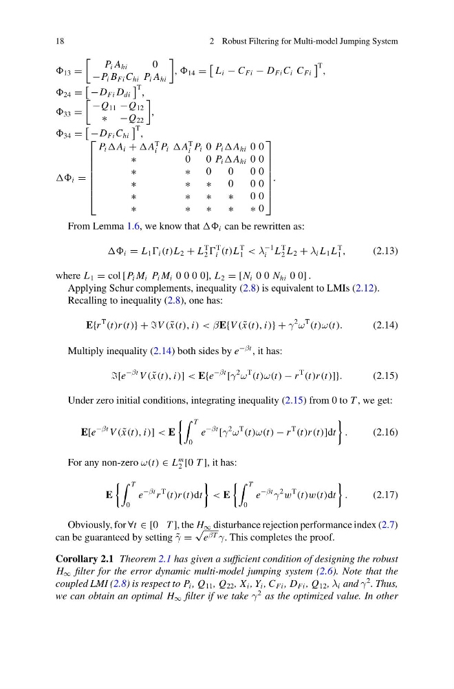
From Lemma 1.6, we know that i can be rewritten as:
i = L 1 i (t)L 2 + L
T
2
T
i (t)L
T
1 < λ
−1
i L
T
2 L 2 + λ i L 1 L
T
1 ,
(2.13)
where L 1 = col [P i M i P i M i 0 0 0 0], L 2 = [N i 0 0 N hi 0 0] .
Applying Schur complements, inequality (2.8) is equivalent to LMIs (2.12).
Recalling to inequality (2.8), one has:
E{r
T
(t)r (t)} + +V ( ˜
x(t), i) < βE{V ( ˜
x(t), i)} + γ
2
ω
T
(t)ω(t).
(2.14)
Multiply inequality (2.14) both sides by e
−βt , it has:
[e
−βt V ( ˜
x(t), i)] < E{e
−βt
[γ
2
ω
T
(t)ω(t) − r
T
(t)r (t)]}.
(2.15)
Under zero initial conditions, integrating inequality (2.15) from 0 to T , we get:
E[e
−βt V ( ˜
x(t), i)] < E
T
0
e
−βt
[γ
2
ω
T
(t)ω(t) − r
T
(t)r (t)]dt
.
(2.16)
For any non-zero ω(t) ∈ L
m
2 [0 T ], it has:
E
T
0
e
−βt r
T
(t)r (t)dt
< E
T
0
e
−βt
γ
2
w
T
(t)w(t)dt
.
(2.17)
Obviously, for ∀t ∈ [0 T ], the H ∞ disturbance rejection performance index (2.7)
can be guaranteed by setting ˜
γ =
√
e βT γ. This completes the proof.
Corollary 2.1 Theorem 2.1 has given a sufficient condition of designing the robust
H ∞ filter for the error dynamic multi-model jumping system (2.6). Note that the
coupled LMI (2.8) is respect to P i , Q 11 , Q 22 , X i , Y i , C Fi , D Fi , Q 12 , λ i and γ
2 . Thus,
we can obtain an optimal H ∞ filter if we take γ
2 as the optimized value. In other
2 Robust Filtering for Multi-model Jumping System
13 =
P i A hi
0
−P i B Fi C hi P i A hi
, 14 =
L i − C Fi − D Fi C i C Fi
T ,
24 =
−D Fi D di
T ,
33 =
−Q 11 −Q 12
∗ −Q 22
,
34 =
−D Fi C hi
T ,
i =
⎡
⎢
⎢
⎢
⎢
⎢
⎢
⎣
P i A i + A
T
i P i A
T
i P i 0 P i A hi 0 0
∗
0
0 P i A hi 0 0
∗
∗
0
0
0 0
∗
∗
∗
0
0 0
∗
∗
∗
∗
0 0
∗
∗
∗
∗
∗ 0
⎤
⎥
⎥
⎥
⎥
⎥
⎥
⎦
.
From Lemma 1.6, we know that i can be rewritten as:
i = L 1 i (t)L 2 + L
T
2
T
i (t)L
T
1 < λ
−1
i L
T
2 L 2 + λ i L 1 L
T
1 ,
(2.13)
where L 1 = col [P i M i P i M i 0 0 0 0], L 2 = [N i 0 0 N hi 0 0] .
Applying Schur complements, inequality (2.8) is equivalent to LMIs (2.12).
Recalling to inequality (2.8), one has:
E{r
T
(t)r (t)} + +V ( ˜
x(t), i) < βE{V ( ˜
x(t), i)} + γ
2
ω
T
(t)ω(t).
(2.14)
Multiply inequality (2.14) both sides by e
−βt , it has:
[e
−βt V ( ˜
x(t), i)] < E{e
−βt
[γ
2
ω
T
(t)ω(t) − r
T
(t)r (t)]}.
(2.15)
Under zero initial conditions, integrating inequality (2.15) from 0 to T , we get:
E[e
−βt V ( ˜
x(t), i)] < E
T
0
e
−βt
[γ
2
ω
T
(t)ω(t) − r
T
(t)r (t)]dt
.
(2.16)
For any non-zero ω(t) ∈ L
m
2 [0 T ], it has:
E
T
0
e
−βt r
T
(t)r (t)dt
< E
T
0
e
−βt
γ
2
w
T
(t)w(t)dt
.
(2.17)
Obviously, for ∀t ∈ [0 T ], the H ∞ disturbance rejection performance index (2.7)
can be guaranteed by setting ˜
γ =
√
e βT γ. This completes the proof.
Corollary 2.1 Theorem 2.1 has given a sufficient condition of designing the robust
H ∞ filter for the error dynamic multi-model jumping system (2.6). Note that the
coupled LMI (2.8) is respect to P i , Q 11 , Q 22 , X i , Y i , C Fi , D Fi , Q 12 , λ i and γ
2 . Thus,
we can obtain an optimal H ∞ filter if we take γ
2 as the optimized value. In other