

9.2 Design of RFD Observer
165
J 1 (T ) = E
T
0
r
T
eo (t)r eo (t) − λ
2
ω
T
(t)ω(t) + +V (e(T ), x(T ), i)
dt
− V (e(T ), x(T ), i)
=
x
T
(t) e
T
(t) x
T
h (t) ω
T
(t)
(X i + i )
(9.21)
x
T
(t) e
T
(t) x
T
h (t) ω
T
(t)
T − V (e(T ), x(T ), i),
where
i =
C i C i C hi + C hi D di + D di
T
C i C i C hi + C hi D di + D di
,
X i =
⎡
⎢
⎢
⎣
1i (A i − H i C i )
T P 2i P 1i (A hi + A hi ) P 1i (B di + B di )
∗
2i
3i
4i
∗
∗
− Q
0
∗
∗
∗
− λ
2 I
⎤
⎥
⎥
⎦ ,
4i = P 2i [B di + B di − H i (D di + D di )].
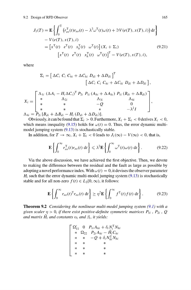
Obviously, it can be found that i > 0. Furthermore, X i + i < 0 derives X i < 0,
which means inequality (9.15) holds for ω(t) = 0. Thus, the error dynamic multimodel jumping system (9.13) is stochastically stable.
In addition, for T → ∞, X i + i < 0 leads to J 1 (∞) − V (∞) < 0, that is,
E
∞
0
r
T
eo (t)r eo (t) dt
λ
2 E
∞
0
ω
T
(t)ω(t) dt
.
(9.22)
Via the above discussion, we have achieved the first objective. Then, we devote
to making the difference between the residual and the fault as large as possible by
adopting a novel performance index. With ω(t) = 0, it devises the observer parameter
H i such that the error dynamic multi-model jumping system (9.13) is stochastically
stable and for all non-zero f (t) ∈ L 2 [0, ∞), it follows:
E
∞
0
r eo (t)
T r eo (t) dt
≥ η
2 E
∞
0
f
T
(t) f (t) dt
.
(9.23)
Theorem 9.2 Considering the nonlinear multi-model jumping system (9.1) with a
given scaler η > 0, if there exist positive-definite symmetric matrices P 1i , P 2i , Q
and matrix ¯
H i and constants α i and β i , it yields:
⎡
⎢
⎢
⎢
⎢
⎢
⎢
⎣
11 0 P 1i A hi + δ i N
T
i N hi
∗ 22 P 2i A hi − ¯
H i C hi
∗ ∗ −Q + δ i N
T
hi N hi
∗ ∗
∗
∗ ∗
∗
∗ ∗
∗
165
J 1 (T ) = E
T
0
r
T
eo (t)r eo (t) − λ
2
ω
T
(t)ω(t) + +V (e(T ), x(T ), i)
dt
− V (e(T ), x(T ), i)
=
x
T
(t) e
T
(t) x
T
h (t) ω
T
(t)
(X i + i )
(9.21)
x
T
(t) e
T
(t) x
T
h (t) ω
T
(t)
T − V (e(T ), x(T ), i),
where
i =
C i C i C hi + C hi D di + D di
T
C i C i C hi + C hi D di + D di
,
X i =
⎡
⎢
⎢
⎣
1i (A i − H i C i )
T P 2i P 1i (A hi + A hi ) P 1i (B di + B di )
∗
2i
3i
4i
∗
∗
− Q
0
∗
∗
∗
− λ
2 I
⎤
⎥
⎥
⎦ ,
4i = P 2i [B di + B di − H i (D di + D di )].
Obviously, it can be found that i > 0. Furthermore, X i + i < 0 derives X i < 0,
which means inequality (9.15) holds for ω(t) = 0. Thus, the error dynamic multimodel jumping system (9.13) is stochastically stable.
In addition, for T → ∞, X i + i < 0 leads to J 1 (∞) − V (∞) < 0, that is,
E
∞
0
r
T
eo (t)r eo (t) dt
λ
2 E
∞
0
ω
T
(t)ω(t) dt
.
(9.22)
Via the above discussion, we have achieved the first objective. Then, we devote
to making the difference between the residual and the fault as large as possible by
adopting a novel performance index. With ω(t) = 0, it devises the observer parameter
H i such that the error dynamic multi-model jumping system (9.13) is stochastically
stable and for all non-zero f (t) ∈ L 2 [0, ∞), it follows:
E
∞
0
r eo (t)
T r eo (t) dt
≥ η
2 E
∞
0
f
T
(t) f (t) dt
.
(9.23)
Theorem 9.2 Considering the nonlinear multi-model jumping system (9.1) with a
given scaler η > 0, if there exist positive-definite symmetric matrices P 1i , P 2i , Q
and matrix ¯
H i and constants α i and β i , it yields:
⎡
⎢
⎢
⎢
⎢
⎢
⎢
⎣
11 0 P 1i A hi + δ i N
T
i N hi
∗ 22 P 2i A hi − ¯
H i C hi
∗ ∗ −Q + δ i N
T
hi N hi
∗ ∗
∗
∗ ∗
∗
∗ ∗
∗