

450
10 Transport Processes
21.5
21.0
20.5
c 0
0
0.5
1.0
1.5
z /cm
Concentration
t 5 4 hours
t 5 2 hours
t 5 1 hour
t 5 0
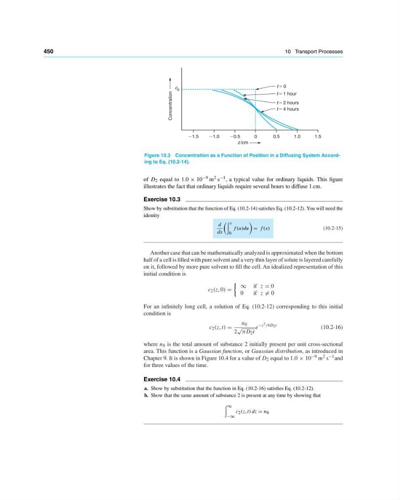
Figure 10.3 Concentration as a Function of Position in a Diffusing System According to Eq. (10.2-14).
of D 2 equal to 1.0 × 10 −9 m 2 s −1 , a typical value for ordinary liquids. This figure
illustrates the fact that ordinary liquids require several hours to diffuse 1 cm.
Exercise 10.3
Show by substitution that the function of Eq. (10.2-14) satisfies Eq. (10.2-12). You will need the
identity
d
dx
x
0
f (u)du
f (x)
(10.2-15)
Another case that can be mathematically analyzed is approximated when the bottom
half of a cell is filled with pure solvent and a very thin layer of solute is layered carefully
on it, followed by more pure solvent to fill the cell. An idealized representation of this
initial condition is
c 2 (z, 0)
∞ if z 0
0
if z 0
For an infinitely long cell, a solution of Eq. (10.2-12) corresponding to this initial
condition is
c 2 (z, t)
n 0
2
√
πD 2 t
e
−z 2 /4D 2 t
(10.2-16)
where n 0 is the total amount of substance 2 initially present per unit cross-sectional
area. This function is a Gaussian function, or Gaussian distribution, as introduced in
Chapter 9. It is shown in Figure 10.4 for a value of D 2 equal to 1.0 × 10 −9 m 2 s −1 and
for three values of the time.
Exercise 10.4
a. Show by substitution that the function in Eq. (10.2-16) satisfies Eq. (10.2-12).
b. Show that the same amount of substance 2 is present at any time by showing that
∞
−∞
c 2 (z, t) dz n 0
10 Transport Processes
21.5
21.0
20.5
c 0
0
0.5
1.0
1.5
z /cm
Concentration
t 5 4 hours
t 5 2 hours
t 5 1 hour
t 5 0
Figure 10.3 Concentration as a Function of Position in a Diffusing System According to Eq. (10.2-14).
of D 2 equal to 1.0 × 10 −9 m 2 s −1 , a typical value for ordinary liquids. This figure
illustrates the fact that ordinary liquids require several hours to diffuse 1 cm.
Exercise 10.3
Show by substitution that the function of Eq. (10.2-14) satisfies Eq. (10.2-12). You will need the
identity
d
dx
x
0
f (u)du
f (x)
(10.2-15)
Another case that can be mathematically analyzed is approximated when the bottom
half of a cell is filled with pure solvent and a very thin layer of solute is layered carefully
on it, followed by more pure solvent to fill the cell. An idealized representation of this
initial condition is
c 2 (z, 0)
∞ if z 0
0
if z 0
For an infinitely long cell, a solution of Eq. (10.2-12) corresponding to this initial
condition is
c 2 (z, t)
n 0
2
√
πD 2 t
e
−z 2 /4D 2 t
(10.2-16)
where n 0 is the total amount of substance 2 initially present per unit cross-sectional
area. This function is a Gaussian function, or Gaussian distribution, as introduced in
Chapter 9. It is shown in Figure 10.4 for a value of D 2 equal to 1.0 × 10 −9 m 2 s −1 and
for three values of the time.
Exercise 10.4
a. Show by substitution that the function in Eq. (10.2-16) satisfies Eq. (10.2-12).
b. Show that the same amount of substance 2 is present at any time by showing that
∞
−∞
c 2 (z, t) dz n 0