

10.2 Transport Processes
451
21.5
21.0
20.5
0
0.5
1.0
1.5
Concentration
z / cm
t 5 4 hours
t 5 2 hours
t 5 1 hour
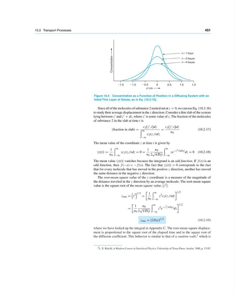
Figure 10.4 Concentration as a Function of Position in a Diffusing System with an
Initial Thin Layer of Solute, as in Eq. (10.2-16).
Since all of the molecules of substance 2 started out at z 0, we can use Eq. (10.2-16)
to study their average displacement in the z direction. Consider a thin slab of the system
lying between z and z + dz, where z is some value of z. The fraction of the molecules
of substance 2 in the slab at time t is
(fraction in slab)
c 2
z , t
dz
∞
−∞
c 2 (z, t)dz
c 2
z , t
dz
n 0
(10.2-17)
The mean value of the coordinate z at time t is given by
z(t)
1
n 0
∞
−∞
zc 2 (z, t)dz 0
1
n 0
n 0
2
√
πD 2 t
∞
−∞
ze
−z 2 /4D 2 t dz 0 (10.2-18)
The mean value z(t) vanishes because the integrand is an odd function. If f (x) is an
odd function, then f (−x) −f (x). The fact that z(t) 0 corresponds to the fact
that for every molecule that has moved in the positive z direction, another has moved
the same distance in the negative z direction.
The root-mean-square value of the z coordinate is a measure of the magnitude of
the distance traveled in the z direction by an average molecule. The root-mean-square
value is the square root of the mean-square value,
z 2
:
z rms
z
2
1/2
1
n 0
∞
−∞
z
2 c 2 (z, t)dz
1/2
1
n 0
n 0
2
√
πD 2 t
∞
−∞
z
2 e
−z 2 /4D 2 t dz
1/2
z rms [2D 2 t]
1/2
(10.2-19)
where we have looked up the integral in Appendix C. The root-mean-square displacement is proportional to the square root of the elapsed time and to the square root of
the diffusion coefficient. This behavior is similar to that of a random walk, 2 which is
2 L. E. Reichl, A Modern Course in Statistical Physics, University of Texas Press, Austin, 1980, p. 151ff.
451
21.5
21.0
20.5
0
0.5
1.0
1.5
Concentration
z / cm
t 5 4 hours
t 5 2 hours
t 5 1 hour
Figure 10.4 Concentration as a Function of Position in a Diffusing System with an
Initial Thin Layer of Solute, as in Eq. (10.2-16).
Since all of the molecules of substance 2 started out at z 0, we can use Eq. (10.2-16)
to study their average displacement in the z direction. Consider a thin slab of the system
lying between z and z + dz, where z is some value of z. The fraction of the molecules
of substance 2 in the slab at time t is
(fraction in slab)
c 2
z , t
dz
∞
−∞
c 2 (z, t)dz
c 2
z , t
dz
n 0
(10.2-17)
The mean value of the coordinate z at time t is given by
z(t)
1
n 0
∞
−∞
zc 2 (z, t)dz 0
1
n 0
n 0
2
√
πD 2 t
∞
−∞
ze
−z 2 /4D 2 t dz 0 (10.2-18)
The mean value z(t) vanishes because the integrand is an odd function. If f (x) is an
odd function, then f (−x) −f (x). The fact that z(t) 0 corresponds to the fact
that for every molecule that has moved in the positive z direction, another has moved
the same distance in the negative z direction.
The root-mean-square value of the z coordinate is a measure of the magnitude of
the distance traveled in the z direction by an average molecule. The root-mean-square
value is the square root of the mean-square value,
z 2
:
z rms
z
2
1/2
1
n 0
∞
−∞
z
2 c 2 (z, t)dz
1/2
1
n 0
n 0
2
√
πD 2 t
∞
−∞
z
2 e
−z 2 /4D 2 t dz
1/2
z rms [2D 2 t]
1/2
(10.2-19)
where we have looked up the integral in Appendix C. The root-mean-square displacement is proportional to the square root of the elapsed time and to the square root of
the diffusion coefficient. This behavior is similar to that of a random walk, 2 which is
2 L. E. Reichl, A Modern Course in Statistical Physics, University of Texas Press, Austin, 1980, p. 151ff.