

10.2 Transport Processes
449
Fick’s Second Law of Diffusion
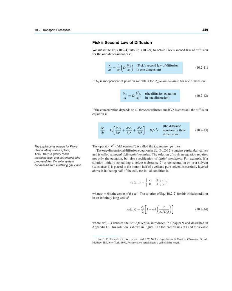
We substitute Eq. (10.2-4) into Eq. (10.2-9) to obtain Fick’s second law of diffusion
for the one-dimensional case:
∂c i
∂t
∂
∂z
D i
∂c i
∂z
(Fick’s second law of diffusion
in one dimension)
(10.2-11)
If D i is independent of position we obtain the diffusion equation for one dimension:
∂c i
∂t
D i
∂ 2 c i
∂z 2
(the diffusion equation
in one dimension)
(10.2-12)
If the concentration depends on all three coordinates and if D i is constant, the diffusion
equation is
∂c i
∂t
D i
∂ 2 c i
∂x 2 +
∂ 2 c i
∂y 2 +
∂ 2 c i
∂z 2
D i ∇ 2 c i
(the diffusion
equation in three
dimensions)
(10.2-13)
The operator ∇ 2 (“del squared”) is called the Laplacian operator.
The Laplacian is named for Pierre
Simon, Marquis de Laplace,
1749–1827, a great French
mathematician and astronomer who
proposed that the solar system
condensed from a rotating gas cloud.
The one-dimensional diffusion equation in Eq. (10.2-12) contains partial derivatives
and is called a partial differential equation. The solution of such an equation requires
not only the equation, but also specification of initial conditions. For example, if a
solution initially containing a solute (substance 2) at concentration c 0 in a solvent
(substance 1) is placed in the bottom half of a cell and pure solvent is carefully layered
above it in the top half of the cell, the initial condition is
c 2 (z, 0)
c 0 if z < 0
0
if z > 0
where z 0 is the center of the cell. The solution of Eq. (10.2-2) for this initial condition
in an infinitely long cell is 1
c 2 (z, t)
c 0
2
1 − erf
z
2
√
D 2 t
(10.2-14)
where erf(· · ·) denotes the error function, introduced in Chapter 9 and described in
Appendix C. This solution is shown in Figure 10.3 for three values of t and for a value
1 See D. P. Shoemaker, C. W. Garland, and J. W. Nibler, Experiments in Physical Chemistry, 6th ed.,
McGraw-Hill, New York, 1996, for a solution pertaining to a cell of finite length.
449
Fick’s Second Law of Diffusion
We substitute Eq. (10.2-4) into Eq. (10.2-9) to obtain Fick’s second law of diffusion
for the one-dimensional case:
∂c i
∂t
∂
∂z
D i
∂c i
∂z
(Fick’s second law of diffusion
in one dimension)
(10.2-11)
If D i is independent of position we obtain the diffusion equation for one dimension:
∂c i
∂t
D i
∂ 2 c i
∂z 2
(the diffusion equation
in one dimension)
(10.2-12)
If the concentration depends on all three coordinates and if D i is constant, the diffusion
equation is
∂c i
∂t
D i
∂ 2 c i
∂x 2 +
∂ 2 c i
∂y 2 +
∂ 2 c i
∂z 2
D i ∇ 2 c i
(the diffusion
equation in three
dimensions)
(10.2-13)
The operator ∇ 2 (“del squared”) is called the Laplacian operator.
The Laplacian is named for Pierre
Simon, Marquis de Laplace,
1749–1827, a great French
mathematician and astronomer who
proposed that the solar system
condensed from a rotating gas cloud.
The one-dimensional diffusion equation in Eq. (10.2-12) contains partial derivatives
and is called a partial differential equation. The solution of such an equation requires
not only the equation, but also specification of initial conditions. For example, if a
solution initially containing a solute (substance 2) at concentration c 0 in a solvent
(substance 1) is placed in the bottom half of a cell and pure solvent is carefully layered
above it in the top half of the cell, the initial condition is
c 2 (z, 0)
c 0 if z < 0
0
if z > 0
where z 0 is the center of the cell. The solution of Eq. (10.2-2) for this initial condition
in an infinitely long cell is 1
c 2 (z, t)
c 0
2
1 − erf
z
2
√
D 2 t
(10.2-14)
where erf(· · ·) denotes the error function, introduced in Chapter 9 and described in
Appendix C. This solution is shown in Figure 10.3 for three values of t and for a value
1 See D. P. Shoemaker, C. W. Garland, and J. W. Nibler, Experiments in Physical Chemistry, 6th ed.,
McGraw-Hill, New York, 1996, for a solution pertaining to a cell of finite length.