

Multiconfigurational Approach to X-ray Spectroscopy …
195
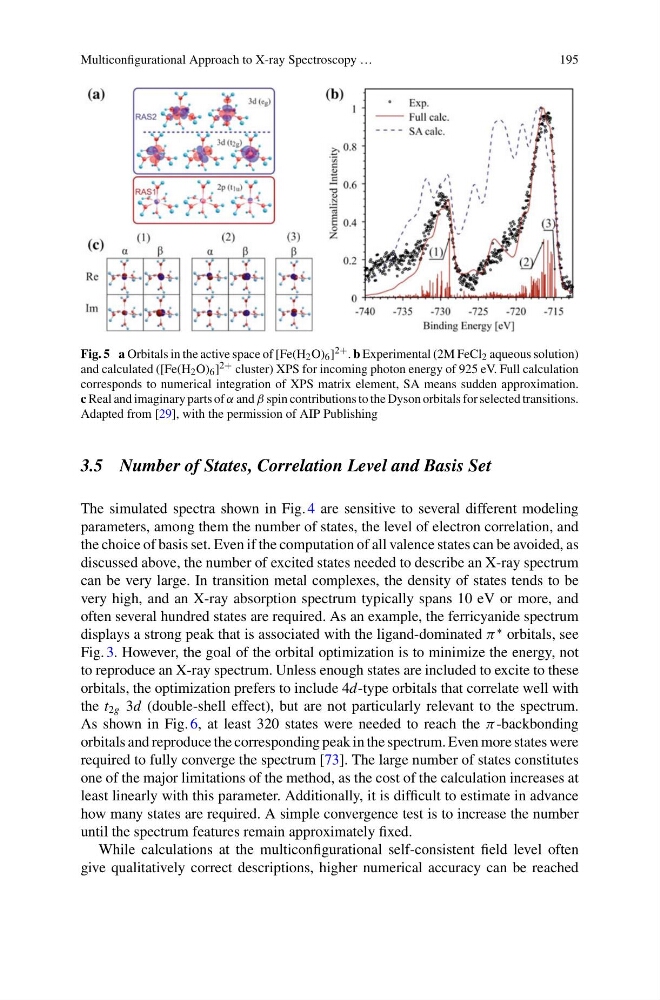
Fig. 5 a Orbitals in the active space of [Fe(H 2 O) 6 ] 2+ . b Experimental (2M FeCl 2 aqueous solution)
and calculated ([Fe(H 2 O) 6 ] 2+ cluster) XPS for incoming photon energy of 925 eV. Full calculation
corresponds to numerical integration of XPS matrix element, SA means sudden approximation.
c Real and imaginary parts of α and β spin contributions to the Dyson orbitals for selected transitions.
Adapted from [29], with the permission of AIP Publishing
3.5 Number of States, Correlation Level and Basis Set
The simulated spectra shown in Fig. 4 are sensitive to several different modeling
parameters, among them the number of states, the level of electron correlation, and
the choice of basis set. Even if the computation of all valence states can be avoided, as
discussed above, the number of excited states needed to describe an X-ray spectrum
can be very large. In transition metal complexes, the density of states tends to be
very high, and an X-ray absorption spectrum typically spans 10 eV or more, and
often several hundred states are required. As an example, the ferricyanide spectrum
displays a strong peak that is associated with the ligand-dominated π
∗ orbitals, see
Fig. 3. However, the goal of the orbital optimization is to minimize the energy, not
to reproduce an X-ray spectrum. Unless enough states are included to excite to these
orbitals, the optimization prefers to include 4d-type orbitals that correlate well with
the t 2g 3d (double-shell effect), but are not particularly relevant to the spectrum.
As shown in Fig. 6, at least 320 states were needed to reach the π -backbonding
orbitals and reproduce the corresponding peak in the spectrum. Even more states were
required to fully converge the spectrum [73]. The large number of states constitutes
one of the major limitations of the method, as the cost of the calculation increases at
least linearly with this parameter. Additionally, it is difficult to estimate in advance
how many states are required. A simple convergence test is to increase the number
until the spectrum features remain approximately fixed.
While calculations at the multiconfigurational self-consistent field level often
give qualitatively correct descriptions, higher numerical accuracy can be reached
195
Fig. 5 a Orbitals in the active space of [Fe(H 2 O) 6 ] 2+ . b Experimental (2M FeCl 2 aqueous solution)
and calculated ([Fe(H 2 O) 6 ] 2+ cluster) XPS for incoming photon energy of 925 eV. Full calculation
corresponds to numerical integration of XPS matrix element, SA means sudden approximation.
c Real and imaginary parts of α and β spin contributions to the Dyson orbitals for selected transitions.
Adapted from [29], with the permission of AIP Publishing
3.5 Number of States, Correlation Level and Basis Set
The simulated spectra shown in Fig. 4 are sensitive to several different modeling
parameters, among them the number of states, the level of electron correlation, and
the choice of basis set. Even if the computation of all valence states can be avoided, as
discussed above, the number of excited states needed to describe an X-ray spectrum
can be very large. In transition metal complexes, the density of states tends to be
very high, and an X-ray absorption spectrum typically spans 10 eV or more, and
often several hundred states are required. As an example, the ferricyanide spectrum
displays a strong peak that is associated with the ligand-dominated π
∗ orbitals, see
Fig. 3. However, the goal of the orbital optimization is to minimize the energy, not
to reproduce an X-ray spectrum. Unless enough states are included to excite to these
orbitals, the optimization prefers to include 4d-type orbitals that correlate well with
the t 2g 3d (double-shell effect), but are not particularly relevant to the spectrum.
As shown in Fig. 6, at least 320 states were needed to reach the π -backbonding
orbitals and reproduce the corresponding peak in the spectrum. Even more states were
required to fully converge the spectrum [73]. The large number of states constitutes
one of the major limitations of the method, as the cost of the calculation increases at
least linearly with this parameter. Additionally, it is difficult to estimate in advance
how many states are required. A simple convergence test is to increase the number
until the spectrum features remain approximately fixed.
While calculations at the multiconfigurational self-consistent field level often
give qualitatively correct descriptions, higher numerical accuracy can be reached