

6.3 Diagrams in Abrikosov Form
91
G
(2)
rs (t 1 , t
+
1 ) = G
(2)
rs (t
+
1 , t 1 ), as will be further discussed in the subsequent chapter.
Since G
(2)
rs (t 1 , t 1 ) is not time-dependent, Eq. (6.17) may be written in the form of a
first-order diagram,
(6.18)
where
X pq = (−i)
rs
V pr[qs] G
(2)
rs (t 1 , t 1 )
(6.19)
represents an effective one-particle potential. As will be discussed in Sect. 8.2, X pq
is a contribution to the static self-energy (SSE) part. In the same way, any diagram
of second and higher order can be inserted in a free fermion line in the form of an
effective potential, symbolically depicted in the following graph:
(6.20)
where the double line stands for any second- or higher-order contribution to G rs (t, t
).
Obviously, such SSE insertions can be made in any free fermion line within a given
diagram. Diagrams with SSE insertions occur for the first time at third order, and they
exhibit necessarily (4–0)-branchings or mergings. This allows us to define ordinary
diagrams more strictly as diagrams which can be brought into a form without any
(4–0)-branchings or mergings.
Matrix Representation of Abrikosov Diagrams
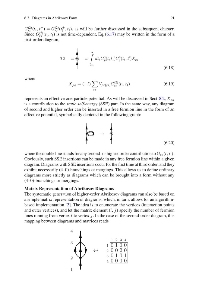
The systematic generation of higher-order Abrikosov diagrams can also be based on
a simple matrix representation of diagrams, which, in turn, allows for an algorithmbased implementation [2]. The idea is to enumerate the vertices (interaction points
and outer vertices), and let the matrix element (i, j) specify the number of fermion
lines running from vertex i to vertex j. In the case of the second-order diagram, this
mapping between diagrams and matrices reads
91
G
(2)
rs (t 1 , t
+
1 ) = G
(2)
rs (t
+
1 , t 1 ), as will be further discussed in the subsequent chapter.
Since G
(2)
rs (t 1 , t 1 ) is not time-dependent, Eq. (6.17) may be written in the form of a
first-order diagram,
(6.18)
where
X pq = (−i)
rs
V pr[qs] G
(2)
rs (t 1 , t 1 )
(6.19)
represents an effective one-particle potential. As will be discussed in Sect. 8.2, X pq
is a contribution to the static self-energy (SSE) part. In the same way, any diagram
of second and higher order can be inserted in a free fermion line in the form of an
effective potential, symbolically depicted in the following graph:
(6.20)
where the double line stands for any second- or higher-order contribution to G rs (t, t
).
Obviously, such SSE insertions can be made in any free fermion line within a given
diagram. Diagrams with SSE insertions occur for the first time at third order, and they
exhibit necessarily (4–0)-branchings or mergings. This allows us to define ordinary
diagrams more strictly as diagrams which can be brought into a form without any
(4–0)-branchings or mergings.
Matrix Representation of Abrikosov Diagrams
The systematic generation of higher-order Abrikosov diagrams can also be based on
a simple matrix representation of diagrams, which, in turn, allows for an algorithmbased implementation [2]. The idea is to enumerate the vertices (interaction points
and outer vertices), and let the matrix element (i, j) specify the number of fermion
lines running from vertex i to vertex j. In the case of the second-order diagram, this
mapping between diagrams and matrices reads