

92
6 Feynman Diagrams
More specifically, the matrix representation of diagrams can be based on the following
rules:
Matrix representation of Abrikosov Diagrams:
(M1) Label the n + 2 vertices by the numbers 1, 2, . . . , n + 2, beginning with the
outer vertex at the bottom (1) and ending with the outer vertex at the top
(n + 2).
(M2) Consider the quadratic (n + 2)-dimensional matrices with entries γ i j =
0, 1, or 2 according to the number of free fermion lines that run from vertex i
to vertex j.
Let us make a few rather obvious observations:
1. Any Abrikosov diagram can be mapped uniquely to a matrix according to (M1)
and (M2): D −→ (D)
2. Different diagrams are mapped to different matrices; that is, the mapping is 1-1
on the domain ({D}).
3. The matrices have the following properties:
(a) The matrix elements in the first column and last row vanish.
(b) Diagonal matrix elements vanish, γ ii = 0.
(c) First row and last column sum up to 1.
(d) Rows and columns associated with inner vertices (2 ≤ i ≤ n + 1) sum up
to 2.
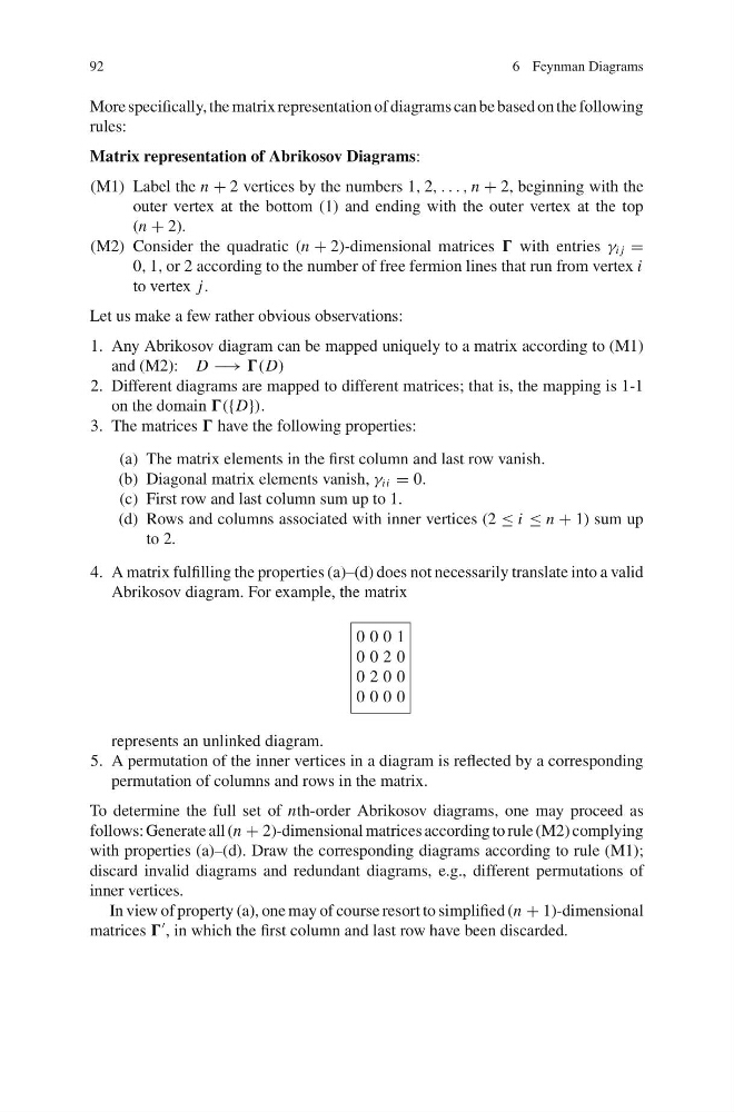
4. A matrix fulfilling the properties (a)–(d) does not necessarily translate into a valid
Abrikosov diagram. For example, the matrix
0 0 0 1
0 0 2 0
0 2 0 0
0 0 0 0
represents an unlinked diagram.
5. A permutation of the inner vertices in a diagram is reflected by a corresponding
permutation of columns and rows in the matrix.
To determine the full set of nth-order Abrikosov diagrams, one may proceed as
follows: Generate all (n + 2)-dimensional matrices according to rule (M2) complying
with properties (a)–(d). Draw the corresponding diagrams according to rule (M1);
discard invalid diagrams and redundant diagrams, e.g., different permutations of
inner vertices.
In view of property (a), one may of course resort to simplified (n + 1)-dimensional
matrices
, in which the first column and last row have been discarded.
6 Feynman Diagrams
More specifically, the matrix representation of diagrams can be based on the following
rules:
Matrix representation of Abrikosov Diagrams:
(M1) Label the n + 2 vertices by the numbers 1, 2, . . . , n + 2, beginning with the
outer vertex at the bottom (1) and ending with the outer vertex at the top
(n + 2).
(M2) Consider the quadratic (n + 2)-dimensional matrices with entries γ i j =
0, 1, or 2 according to the number of free fermion lines that run from vertex i
to vertex j.
Let us make a few rather obvious observations:
1. Any Abrikosov diagram can be mapped uniquely to a matrix according to (M1)
and (M2): D −→ (D)
2. Different diagrams are mapped to different matrices; that is, the mapping is 1-1
on the domain ({D}).
3. The matrices have the following properties:
(a) The matrix elements in the first column and last row vanish.
(b) Diagonal matrix elements vanish, γ ii = 0.
(c) First row and last column sum up to 1.
(d) Rows and columns associated with inner vertices (2 ≤ i ≤ n + 1) sum up
to 2.
4. A matrix fulfilling the properties (a)–(d) does not necessarily translate into a valid
Abrikosov diagram. For example, the matrix
0 0 0 1
0 0 2 0
0 2 0 0
0 0 0 0
represents an unlinked diagram.
5. A permutation of the inner vertices in a diagram is reflected by a corresponding
permutation of columns and rows in the matrix.
To determine the full set of nth-order Abrikosov diagrams, one may proceed as
follows: Generate all (n + 2)-dimensional matrices according to rule (M2) complying
with properties (a)–(d). Draw the corresponding diagrams according to rule (M1);
discard invalid diagrams and redundant diagrams, e.g., different permutations of
inner vertices.
In view of property (a), one may of course resort to simplified (n + 1)-dimensional
matrices
, in which the first column and last row have been discarded.