

90
6 Feynman Diagrams
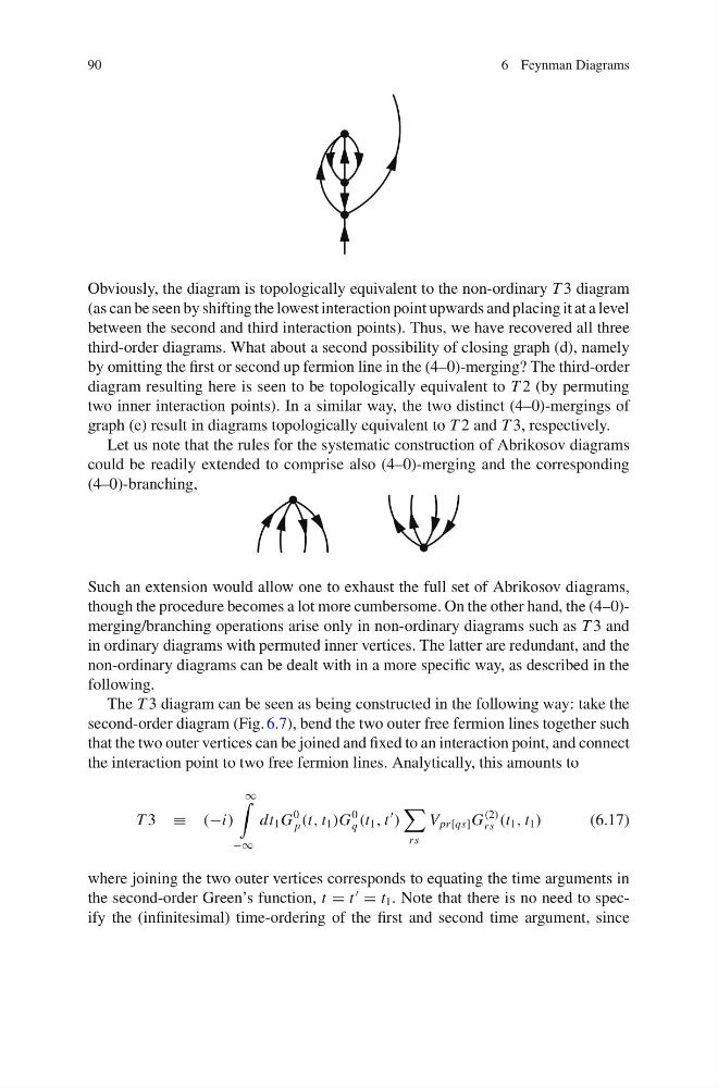
Obviously, the diagram is topologically equivalent to the non-ordinary T 3 diagram
(as can be seen by shifting the lowest interaction point upwards and placing it at a level
between the second and third interaction points). Thus, we have recovered all three
third-order diagrams. What about a second possibility of closing graph (d), namely
by omitting the first or second up fermion line in the (4–0)-merging? The third-order
diagram resulting here is seen to be topologically equivalent to T 2 (by permuting
two inner interaction points). In a similar way, the two distinct (4–0)-mergings of
graph (e) result in diagrams topologically equivalent to T 2 and T 3, respectively.
Let us note that the rules for the systematic construction of Abrikosov diagrams
could be readily extended to comprise also (4–0)-merging and the corresponding
(4–0)-branching,
Such an extension would allow one to exhaust the full set of Abrikosov diagrams,
though the procedure becomes a lot more cumbersome. On the other hand, the (4–0)merging/branching operations arise only in non-ordinary diagrams such as T 3 and
in ordinary diagrams with permuted inner vertices. The latter are redundant, and the
non-ordinary diagrams can be dealt with in a more specific way, as described in the
following.
The T 3 diagram can be seen as being constructed in the following way: take the
second-order diagram (Fig. 6.7), bend the two outer free fermion lines together such
that the two outer vertices can be joined and fixed to an interaction point, and connect
the interaction point to two free fermion lines. Analytically, this amounts to
T 3 ≡ (−i)
∞
−∞
dt 1 G
0
p (t, t 1 )G
0
q (t 1 , t
)
rs
V pr[qs] G
(2)
rs (t 1 , t 1 )
(6.17)
where joining the two outer vertices corresponds to equating the time arguments in
the second-order Green’s function, t = t
= t 1 . Note that there is no need to specify the (infinitesimal) time-ordering of the first and second time argument, since
6 Feynman Diagrams
Obviously, the diagram is topologically equivalent to the non-ordinary T 3 diagram
(as can be seen by shifting the lowest interaction point upwards and placing it at a level
between the second and third interaction points). Thus, we have recovered all three
third-order diagrams. What about a second possibility of closing graph (d), namely
by omitting the first or second up fermion line in the (4–0)-merging? The third-order
diagram resulting here is seen to be topologically equivalent to T 2 (by permuting
two inner interaction points). In a similar way, the two distinct (4–0)-mergings of
graph (e) result in diagrams topologically equivalent to T 2 and T 3, respectively.
Let us note that the rules for the systematic construction of Abrikosov diagrams
could be readily extended to comprise also (4–0)-merging and the corresponding
(4–0)-branching,
Such an extension would allow one to exhaust the full set of Abrikosov diagrams,
though the procedure becomes a lot more cumbersome. On the other hand, the (4–0)merging/branching operations arise only in non-ordinary diagrams such as T 3 and
in ordinary diagrams with permuted inner vertices. The latter are redundant, and the
non-ordinary diagrams can be dealt with in a more specific way, as described in the
following.
The T 3 diagram can be seen as being constructed in the following way: take the
second-order diagram (Fig. 6.7), bend the two outer free fermion lines together such
that the two outer vertices can be joined and fixed to an interaction point, and connect
the interaction point to two free fermion lines. Analytically, this amounts to
T 3 ≡ (−i)
∞
−∞
dt 1 G
0
p (t, t 1 )G
0
q (t 1 , t
)
rs
V pr[qs] G
(2)
rs (t 1 , t 1 )
(6.17)
where joining the two outer vertices corresponds to equating the time arguments in
the second-order Green’s function, t = t
= t 1 . Note that there is no need to specify the (infinitesimal) time-ordering of the first and second time argument, since