

6.3 Diagrams in Abrikosov Form
89
4. Finally, check whether there are topologically equivalent diagrams (e.g., two diagrams differing only in a permutation of interaction points) and discard redundant
diagrams.
Let us use these recipes through third order. At the order level n = 1, there is just
the initial (1–3)-branching
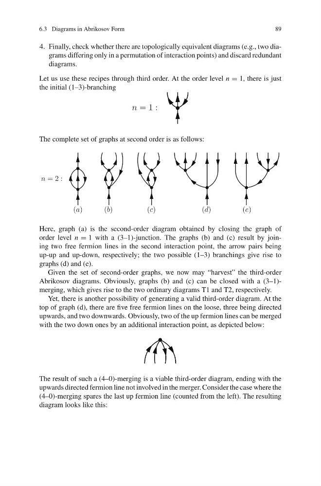
The complete set of graphs at second order is as follows:
Here, graph (a) is the second-order diagram obtained by closing the graph of
order level n = 1 with a (3–1)-junction. The graphs (b) and (c) result by joining two free fermion lines in the second interaction point, the arrow pairs being
up-up and up-down, respectively; the two possible (1–3) branchings give rise to
graphs (d) and (e).
Given the set of second-order graphs, we now may “harvest” the third-order
Abrikosov diagrams. Obviously, graphs (b) and (c) can be closed with a (3–1)merging, which gives rise to the two ordinary diagrams T1 and T2, respectively.
Yet, there is another possibility of generating a valid third-order diagram. At the
top of graph (d), there are five free fermion lines on the loose, three being directed
upwards, and two downwards. Obviously, two of the up fermion lines can be merged
with the two down ones by an additional interaction point, as depicted below:
The result of such a (4–0)-merging is a viable third-order diagram, ending with the
upwards directed fermion line not involved in the merger. Consider the case where the
(4–0)-merging spares the last up fermion line (counted from the left). The resulting
diagram looks like this:
89
4. Finally, check whether there are topologically equivalent diagrams (e.g., two diagrams differing only in a permutation of interaction points) and discard redundant
diagrams.
Let us use these recipes through third order. At the order level n = 1, there is just
the initial (1–3)-branching
The complete set of graphs at second order is as follows:
Here, graph (a) is the second-order diagram obtained by closing the graph of
order level n = 1 with a (3–1)-junction. The graphs (b) and (c) result by joining two free fermion lines in the second interaction point, the arrow pairs being
up-up and up-down, respectively; the two possible (1–3) branchings give rise to
graphs (d) and (e).
Given the set of second-order graphs, we now may “harvest” the third-order
Abrikosov diagrams. Obviously, graphs (b) and (c) can be closed with a (3–1)merging, which gives rise to the two ordinary diagrams T1 and T2, respectively.
Yet, there is another possibility of generating a valid third-order diagram. At the
top of graph (d), there are five free fermion lines on the loose, three being directed
upwards, and two downwards. Obviously, two of the up fermion lines can be merged
with the two down ones by an additional interaction point, as depicted below:
The result of such a (4–0)-merging is a viable third-order diagram, ending with the
upwards directed fermion line not involved in the merger. Consider the case where the
(4–0)-merging spares the last up fermion line (counted from the left). The resulting
diagram looks like this: