

88
6 Feynman Diagrams
Systematic Construction of Abrikosov Diagrams
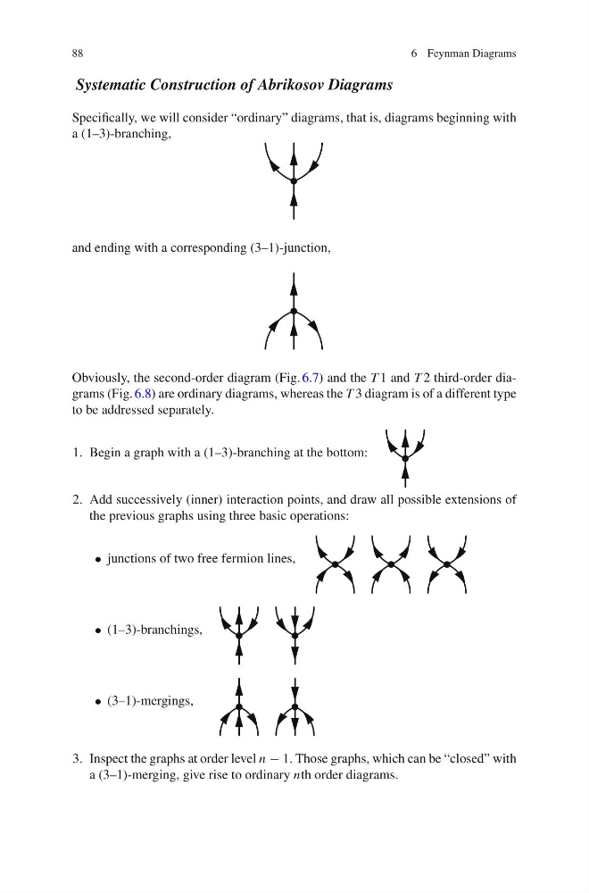
Specifically, we will consider “ordinary” diagrams, that is, diagrams beginning with
a (1–3)-branching,
and ending with a corresponding (3–1)-junction,
Obviously, the second-order diagram (Fig. 6.7) and the T 1 and T 2 third-order diagrams (Fig. 6.8) are ordinary diagrams, whereas the T 3 diagram is of a different type
to be addressed separately.
1. Begin a graph with a (1–3)-branching at the bottom:
2. Add successively (inner) interaction points, and draw all possible extensions of
the previous graphs using three basic operations:
• junctions of two free fermion lines,
• (1–3)-branchings,
• (3–1)-mergings,
3. Inspect the graphs at order level n − 1. Those graphs, which can be “closed” with
a (3–1)-merging, give rise to ordinary nth order diagrams.
6 Feynman Diagrams
Systematic Construction of Abrikosov Diagrams
Specifically, we will consider “ordinary” diagrams, that is, diagrams beginning with
a (1–3)-branching,
and ending with a corresponding (3–1)-junction,
Obviously, the second-order diagram (Fig. 6.7) and the T 1 and T 2 third-order diagrams (Fig. 6.8) are ordinary diagrams, whereas the T 3 diagram is of a different type
to be addressed separately.
1. Begin a graph with a (1–3)-branching at the bottom:
2. Add successively (inner) interaction points, and draw all possible extensions of
the previous graphs using three basic operations:
• junctions of two free fermion lines,
• (1–3)-branchings,
• (3–1)-mergings,
3. Inspect the graphs at order level n − 1. Those graphs, which can be “closed” with
a (3–1)-merging, give rise to ordinary nth order diagrams.