

6.3 Diagrams in Abrikosov Form
87
Rules for Abrikosov Diagrams
(A1) Draw all topologically distinct connected diagrams with n interaction dots
and 2n + 1 directed (solid) free Green’s function or G
0 -lines starting at the
outer vertex (q, t
) and ending at the outer vertex ( p, t). At each interaction
dot, two G
0 -lines start and two G
0 -lines end; assign a time argument to each
interaction dot.
(A2) Attach one-particle indices and time arguments to the G
0 -lines; the arrows
define the order of the time arguments. Replace the graphical symbols (free
fermion lines and interaction dots) by the respective analytical expressions.
(A3) Sum over indices and integrate over time arguments of the inner vertices.
(A4) The overall phase of an Abrikosov diagram can only be fixed by inspecting one
of the Feynman diagrams comprised in the Abrikosov diagram. The phase is
to be adapted in such a way that this Feynman diagram is reproduced correctly
by the Abrikosov expression.
(A5) Apply a factor of
1
2
for each pair of (topologically) equivalent G
0 -lines to
compensate for double counting of Feynman diagrams. Double counting may
arise for other reasons at fourth and higher order, and this possibility must be
checked at the level of Feynman diagrams.
As we have already seen, there is a single second-order Abrikosov diagram
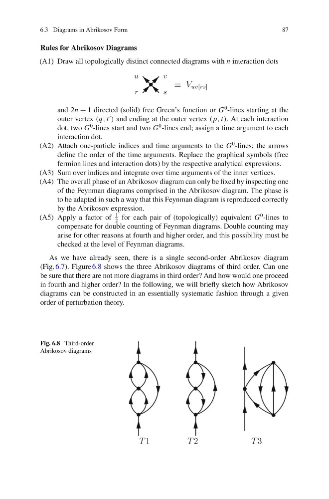
(Fig. 6.7). Figure 6.8 shows the three Abrikosov diagrams of third order. Can one
be sure that there are not more diagrams in third order? And how would one proceed
in fourth and higher order? In the following, we will briefly sketch how Abrikosov
diagrams can be constructed in an essentially systematic fashion through a given
order of perturbation theory.
Fig. 6.8 Third-order
Abrikosov diagrams
87
Rules for Abrikosov Diagrams
(A1) Draw all topologically distinct connected diagrams with n interaction dots
and 2n + 1 directed (solid) free Green’s function or G
0 -lines starting at the
outer vertex (q, t
) and ending at the outer vertex ( p, t). At each interaction
dot, two G
0 -lines start and two G
0 -lines end; assign a time argument to each
interaction dot.
(A2) Attach one-particle indices and time arguments to the G
0 -lines; the arrows
define the order of the time arguments. Replace the graphical symbols (free
fermion lines and interaction dots) by the respective analytical expressions.
(A3) Sum over indices and integrate over time arguments of the inner vertices.
(A4) The overall phase of an Abrikosov diagram can only be fixed by inspecting one
of the Feynman diagrams comprised in the Abrikosov diagram. The phase is
to be adapted in such a way that this Feynman diagram is reproduced correctly
by the Abrikosov expression.
(A5) Apply a factor of
1
2
for each pair of (topologically) equivalent G
0 -lines to
compensate for double counting of Feynman diagrams. Double counting may
arise for other reasons at fourth and higher order, and this possibility must be
checked at the level of Feynman diagrams.
As we have already seen, there is a single second-order Abrikosov diagram
(Fig. 6.7). Figure 6.8 shows the three Abrikosov diagrams of third order. Can one
be sure that there are not more diagrams in third order? And how would one proceed
in fourth and higher order? In the following, we will briefly sketch how Abrikosov
diagrams can be constructed in an essentially systematic fashion through a given
order of perturbation theory.
Fig. 6.8 Third-order
Abrikosov diagrams