

6.3 Diagrams in Abrikosov Form
85
showing a wiggly interaction line (≡ V i jrs ) with its four free fermion lines. The
letters A, B, C, and D indicate the clipped connections to the rest of the diagram.
The fermion line D → A on the left side of the vertex is part of an extended fermion
line, being either a continuous line or a closed loop, and the same applies to C → B
on the right-hand side. Exchanging the two incoming free fermion lines as indicated
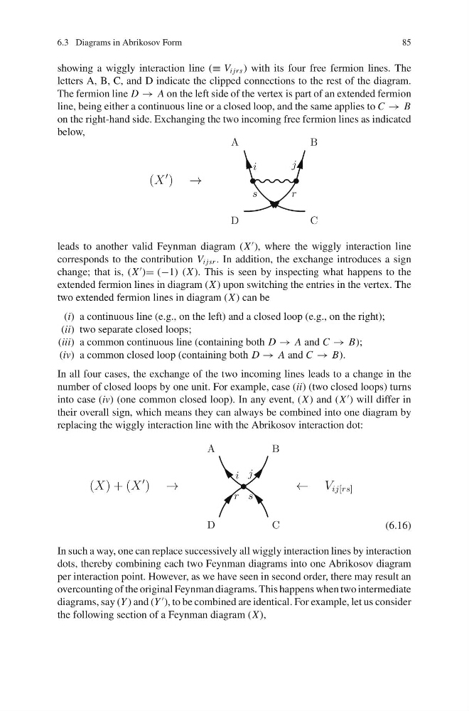
below,
leads to another valid Feynman diagram (X
), where the wiggly interaction line
corresponds to the contribution V i jsr . In addition, the exchange introduces a sign
change; that is, (X
)= (−1) (X ). This is seen by inspecting what happens to the
extended fermion lines in diagram (X ) upon switching the entries in the vertex. The
two extended fermion lines in diagram (X ) can be
(i) a continuous line (e.g., on the left) and a closed loop (e.g., on the right);
(ii) two separate closed loops;
(iii) a common continuous line (containing both D → A and C → B);
(iv) a common closed loop (containing both D → A and C → B).
In all four cases, the exchange of the two incoming lines leads to a change in the
number of closed loops by one unit. For example, case (ii) (two closed loops) turns
into case (iv) (one common closed loop). In any event, (X ) and (X
) will differ in
their overall sign, which means they can always be combined into one diagram by
replacing the wiggly interaction line with the Abrikosov interaction dot:
(6.16)
In such a way, one can replace successively all wiggly interaction lines by interaction
dots, thereby combining each two Feynman diagrams into one Abrikosov diagram
per interaction point. However, as we have seen in second order, there may result an
overcounting of the original Feynman diagrams. This happens when two intermediate
diagrams, say (Y ) and (Y
), to be combined are identical. For example, let us consider
the following section of a Feynman diagram (X ),
85
showing a wiggly interaction line (≡ V i jrs ) with its four free fermion lines. The
letters A, B, C, and D indicate the clipped connections to the rest of the diagram.
The fermion line D → A on the left side of the vertex is part of an extended fermion
line, being either a continuous line or a closed loop, and the same applies to C → B
on the right-hand side. Exchanging the two incoming free fermion lines as indicated
below,
leads to another valid Feynman diagram (X
), where the wiggly interaction line
corresponds to the contribution V i jsr . In addition, the exchange introduces a sign
change; that is, (X
)= (−1) (X ). This is seen by inspecting what happens to the
extended fermion lines in diagram (X ) upon switching the entries in the vertex. The
two extended fermion lines in diagram (X ) can be
(i) a continuous line (e.g., on the left) and a closed loop (e.g., on the right);
(ii) two separate closed loops;
(iii) a common continuous line (containing both D → A and C → B);
(iv) a common closed loop (containing both D → A and C → B).
In all four cases, the exchange of the two incoming lines leads to a change in the
number of closed loops by one unit. For example, case (ii) (two closed loops) turns
into case (iv) (one common closed loop). In any event, (X ) and (X
) will differ in
their overall sign, which means they can always be combined into one diagram by
replacing the wiggly interaction line with the Abrikosov interaction dot:
(6.16)
In such a way, one can replace successively all wiggly interaction lines by interaction
dots, thereby combining each two Feynman diagrams into one Abrikosov diagram
per interaction point. However, as we have seen in second order, there may result an
overcounting of the original Feynman diagrams. This happens when two intermediate
diagrams, say (Y ) and (Y
), to be combined are identical. For example, let us consider
the following section of a Feynman diagram (X ),