

84
6 Feynman Diagrams
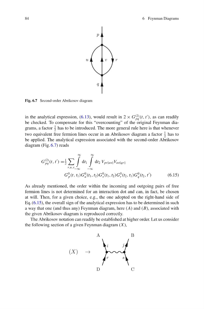
Fig. 6.7 Second-order Abrikosov diagram
in the analytical expression, (6.13), would result in 2 × G
(2)
pq (t, t
), as can readily
be checked. To compensate for this “overcounting” of the original Feynman diagrams, a factor
1
2
has to be introduced. The more general rule here is that whenever
two equivalent free fermion lines occur in an Abrikosov diagram a factor
1
2
has to
be applied. The analytical expression associated with the second-order Abrikosov
diagram (Fig. 6.7) reads
G
(2)
pq (t, t
) =
1
2
r,u,v
∞
−∞
dt 1
∞
−∞
dt 2 V pr[uv] V uv[qr]
G
0
p (t, t 1 )G
0
u (t 1 , t 2 )G
0
v (t 1 , t 2 )G
0
r (t 2 , t 1 )G
0
q (t 2 , t
)
(6.15)
As already mentioned, the order within the incoming and outgoing pairs of free
fermion lines is not determined for an interaction dot and can, in fact, be chosen
at will. Then, for a given choice, e.g., the one adopted on the right-hand side of
Eq. (6.15), the overall sign of the analytical expression has to be determined in such
a way that one (and thus any) Feynman diagram, here ( A) and (B), associated with
the given Abrikosov diagram is reproduced correctly.
The Abrikosov notation can readily be established at higher order. Let us consider
the following section of a given Feynman diagram (X ),
6 Feynman Diagrams
Fig. 6.7 Second-order Abrikosov diagram
in the analytical expression, (6.13), would result in 2 × G
(2)
pq (t, t
), as can readily
be checked. To compensate for this “overcounting” of the original Feynman diagrams, a factor
1
2
has to be introduced. The more general rule here is that whenever
two equivalent free fermion lines occur in an Abrikosov diagram a factor
1
2
has to
be applied. The analytical expression associated with the second-order Abrikosov
diagram (Fig. 6.7) reads
G
(2)
pq (t, t
) =
1
2
r,u,v
∞
−∞
dt 1
∞
−∞
dt 2 V pr[uv] V uv[qr]
G
0
p (t, t 1 )G
0
u (t 1 , t 2 )G
0
v (t 1 , t 2 )G
0
r (t 2 , t 1 )G
0
q (t 2 , t
)
(6.15)
As already mentioned, the order within the incoming and outgoing pairs of free
fermion lines is not determined for an interaction dot and can, in fact, be chosen
at will. Then, for a given choice, e.g., the one adopted on the right-hand side of
Eq. (6.15), the overall sign of the analytical expression has to be determined in such
a way that one (and thus any) Feynman diagram, here ( A) and (B), associated with
the given Abrikosov diagram is reproduced correctly.
The Abrikosov notation can readily be established at higher order. Let us consider
the following section of a given Feynman diagram (X ),