

6.2 Diagrams in the Hartree–Fock Representation
83
Here, the individual contributions ( A) and (B) correspond to the two terms obtained
by expanding the round brackets.
6.3 Diagrams in Abrikosov Form
The bracket on the right-hand side of Eq. (6.13) could have been written in a more
compact form according to
(V pruv − V prvu )V uvqr = V pr[uv] V uvqr
where the antisymmetrized Coulomb integral V pr[uv] combines the integral terms
of the ( A) and (B) diagrams. This suggests to introduce a corresponding graphical
symbol,
(6.14)
referred to as the (two-particle) interaction dot. As will be discussed below, it is
possible to replace the original Feynman diagrams by diagrams in Abrikosov notation [1] (or simply Abrikosov diagrams) using interaction dots rather than wiggly
lines. Obviously, an interaction dot does not determine the sign of the associated
antisymmetrized Coulomb integral since the order of the two incoming or two outgoing fermion lines is ambiguous. As a consequence, the overall sign of an Abrikosov
diagram can only be defined by resorting to one of the underlying Feynman diagrams.
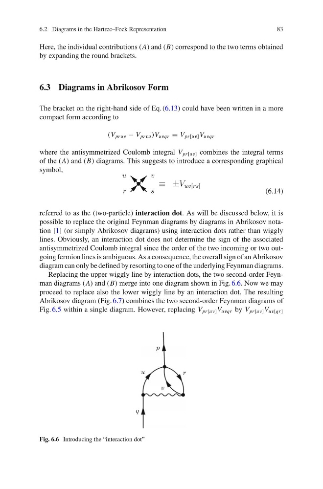
Replacing the upper wiggly line by interaction dots, the two second-order Feynman diagrams (A) and (B) merge into one diagram shown in Fig. 6.6. Now we may
proceed to replace also the lower wiggly line by an interaction dot. The resulting
Abrikosov diagram (Fig. 6.7) combines the two second-order Feynman diagrams of
Fig. 6.5 within a single diagram. However, replacing V pr[uv] V uvqr by V pr[uv] V uv[qr]
Fig. 6.6 Introducing the “interaction dot”
83
Here, the individual contributions ( A) and (B) correspond to the two terms obtained
by expanding the round brackets.
6.3 Diagrams in Abrikosov Form
The bracket on the right-hand side of Eq. (6.13) could have been written in a more
compact form according to
(V pruv − V prvu )V uvqr = V pr[uv] V uvqr
where the antisymmetrized Coulomb integral V pr[uv] combines the integral terms
of the ( A) and (B) diagrams. This suggests to introduce a corresponding graphical
symbol,
(6.14)
referred to as the (two-particle) interaction dot. As will be discussed below, it is
possible to replace the original Feynman diagrams by diagrams in Abrikosov notation [1] (or simply Abrikosov diagrams) using interaction dots rather than wiggly
lines. Obviously, an interaction dot does not determine the sign of the associated
antisymmetrized Coulomb integral since the order of the two incoming or two outgoing fermion lines is ambiguous. As a consequence, the overall sign of an Abrikosov
diagram can only be defined by resorting to one of the underlying Feynman diagrams.
Replacing the upper wiggly line by interaction dots, the two second-order Feynman diagrams (A) and (B) merge into one diagram shown in Fig. 6.6. Now we may
proceed to replace also the lower wiggly line by an interaction dot. The resulting
Abrikosov diagram (Fig. 6.7) combines the two second-order Feynman diagrams of
Fig. 6.5 within a single diagram. However, replacing V pr[uv] V uvqr by V pr[uv] V uv[qr]
Fig. 6.6 Introducing the “interaction dot”