

82
6 Feynman Diagrams
s rs = w rs +
v
V r v[sv] n v
(6.10)
According to Eq. (4.6), the matrix elements of the one-particle interaction part are
given by
w rs = −
v
V r v[sv] n v
which means that the effective first-order matrix elements simply vanish,
s rs = 0
(6.11)
As a consequence, any diagram containing a one-particle cross, or an oyster, or a
tadpole part can be discarded. In particular, the first-order contribution to the electron
propagator vanishes:
G
(1)
pq (t, t
) = 0
(6.12)
so that the perturbation expansion through second order becomes
G pq (t, t
) = G
0
pq (t, t
) + G
(2)
pq (t, t
) + O(3)
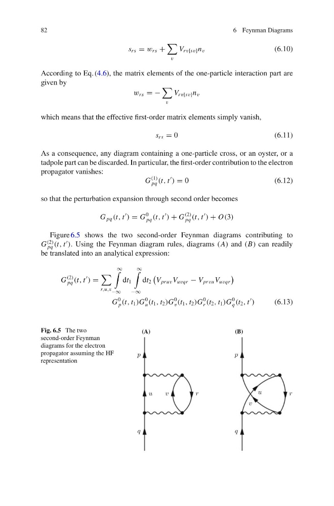
Figure 6.5 shows the two second-order Feynman diagrams contributing to
G
(2)
pq (t, t
). Using the Feynman diagram rules, diagrams (A) and (B) can readily
be translated into an analytical expression:
G
(2)
pq (t, t
) =
r,u,v
∞
−∞
dt 1
∞
−∞
dt 2
V pruv V uvqr − V prvu V uvqr
G
0
p (t, t 1 )G
0
u (t 1 , t 2 )G
0
v (t 1 , t 2 )G
0
r (t 2 , t 1 )G
0
q (t 2 , t
)
(6.13)
Fig. 6.5 The two
second-order Feynman
diagrams for the electron
propagator assuming the HF
representation
(A)
(B)
6 Feynman Diagrams
s rs = w rs +
v
V r v[sv] n v
(6.10)
According to Eq. (4.6), the matrix elements of the one-particle interaction part are
given by
w rs = −
v
V r v[sv] n v
which means that the effective first-order matrix elements simply vanish,
s rs = 0
(6.11)
As a consequence, any diagram containing a one-particle cross, or an oyster, or a
tadpole part can be discarded. In particular, the first-order contribution to the electron
propagator vanishes:
G
(1)
pq (t, t
) = 0
(6.12)
so that the perturbation expansion through second order becomes
G pq (t, t
) = G
0
pq (t, t
) + G
(2)
pq (t, t
) + O(3)
Figure 6.5 shows the two second-order Feynman diagrams contributing to
G
(2)
pq (t, t
). Using the Feynman diagram rules, diagrams (A) and (B) can readily
be translated into an analytical expression:
G
(2)
pq (t, t
) =
r,u,v
∞
−∞
dt 1
∞
−∞
dt 2
V pruv V uvqr − V prvu V uvqr
G
0
p (t, t 1 )G
0
u (t 1 , t 2 )G
0
v (t 1 , t 2 )G
0
r (t 2 , t 1 )G
0
q (t 2 , t
)
(6.13)
Fig. 6.5 The two
second-order Feynman
diagrams for the electron
propagator assuming the HF
representation
(A)
(B)