

6.1 Second-Order Diagrams
77
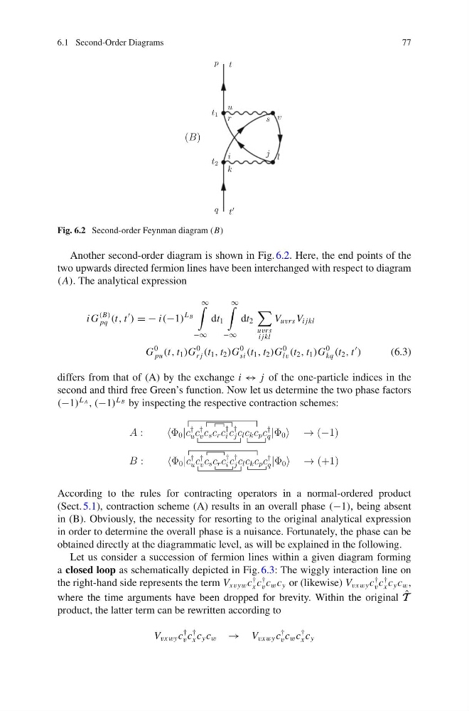
Fig. 6.2 Second-order Feynman diagram (B)
Another second-order diagram is shown in Fig. 6.2. Here, the end points of the
two upwards directed fermion lines have been interchanged with respect to diagram
(A). The analytical expression
i G
(B)
pq (t, t
) = − i(−1)
L B
∞
−∞
dt 1
∞
−∞
dt 2
uvrs
i jkl
V uvrs V i jkl
G
0
pu (t, t 1 )G
0
r j (t 1 , t 2 )G
0
si (t 1 , t 2 )G
0
lv (t 2 , t 1 )G
0
kq (t 2 , t
)
(6.3)
differs from that of (A) by the exchange i ↔ j of the one-particle indices in the
second and third free Green’s function. Now let us determine the two phase factors
(−1)
L A , (−1)
L B by inspecting the respective contraction schemes:
According to the rules for contracting operators in a normal-ordered product
(Sect. 5.1), contraction scheme (A) results in an overall phase (−1), being absent
in (B). Obviously, the necessity for resorting to the original analytical expression
in order to determine the overall phase is a nuisance. Fortunately, the phase can be
obtained directly at the diagrammatic level, as will be explained in the following.
Let us consider a succession of fermion lines within a given diagram forming
a closed loop as schematically depicted in Fig. 6.3: The wiggly interaction line on
the right-hand side represents the term V xvyw c
†
x c
†
v c w c y or (likewise) V vxwy c
†
v c
†
x c y c w ,
where the time arguments have been dropped for brevity. Within the original ˆ
T T T
product, the latter term can be rewritten according to
V vxwy c
†
v c
†
x c y c w → V vxwy c
†
v c w c
†
x c y
77
Fig. 6.2 Second-order Feynman diagram (B)
Another second-order diagram is shown in Fig. 6.2. Here, the end points of the
two upwards directed fermion lines have been interchanged with respect to diagram
(A). The analytical expression
i G
(B)
pq (t, t
) = − i(−1)
L B
∞
−∞
dt 1
∞
−∞
dt 2
uvrs
i jkl
V uvrs V i jkl
G
0
pu (t, t 1 )G
0
r j (t 1 , t 2 )G
0
si (t 1 , t 2 )G
0
lv (t 2 , t 1 )G
0
kq (t 2 , t
)
(6.3)
differs from that of (A) by the exchange i ↔ j of the one-particle indices in the
second and third free Green’s function. Now let us determine the two phase factors
(−1)
L A , (−1)
L B by inspecting the respective contraction schemes:
According to the rules for contracting operators in a normal-ordered product
(Sect. 5.1), contraction scheme (A) results in an overall phase (−1), being absent
in (B). Obviously, the necessity for resorting to the original analytical expression
in order to determine the overall phase is a nuisance. Fortunately, the phase can be
obtained directly at the diagrammatic level, as will be explained in the following.
Let us consider a succession of fermion lines within a given diagram forming
a closed loop as schematically depicted in Fig. 6.3: The wiggly interaction line on
the right-hand side represents the term V xvyw c
†
x c
†
v c w c y or (likewise) V vxwy c
†
v c
†
x c y c w ,
where the time arguments have been dropped for brevity. Within the original ˆ
T T T
product, the latter term can be rewritten according to
V vxwy c
†
v c
†
x c y c w → V vxwy c
†
v c w c
†
x c y