

48
4 Perturbation Theory for the Electron Propagator
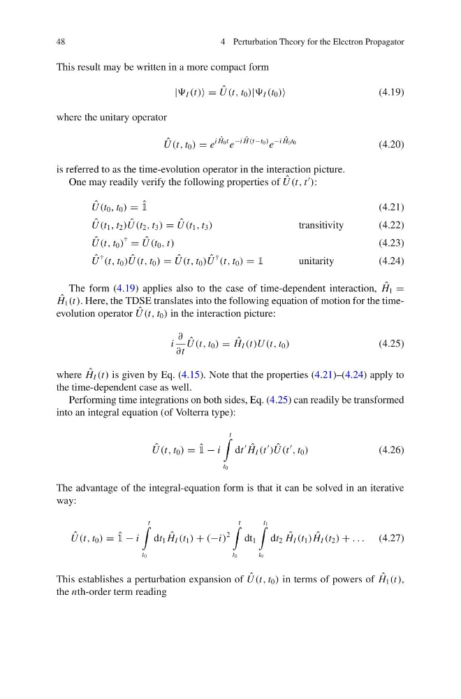
This result may be written in a more compact form
| I (t) = ˆ
U (t, t 0 )| I (t 0 )
(4.19)
where the unitary operator
ˆ
U (t, t 0 ) = e
i ˆ
H 0 t e
−i ˆ
H (t−t 0 ) e
−i ˆ
H 0 t 0
(4.20)
is referred to as the time-evolution operator in the interaction picture.
One may readily verify the following properties of ˆ
U (t, t
):
ˆ
U (t 0 , t 0 ) = ˆ
1
(4.21)
ˆ
U (t 1 , t 2 ) ˆ
U (t 2 , t 3 ) = ˆ
U (t 1 , t 3 )
transitivity
(4.22)
ˆ
U (t, t 0 )
†
= ˆ
U (t 0 , t)
(4.23)
ˆ
U
†
(t, t 0 ) ˆ
U (t, t 0 ) = ˆ
U (t, t 0 ) ˆ
U
†
(t, t 0 ) = 1
unitarity
(4.24)
The form (4.19) applies also to the case of time-dependent interaction, ˆ
H 1 =
ˆ
H 1 (t). Here, the TDSE translates into the following equation of motion for the timeevolution operator ˆ
U (t, t 0 ) in the interaction picture:
i
∂
∂t
ˆ
U (t, t 0 ) = ˆ
H I (t)U (t, t 0 )
(4.25)
where ˆ
H I (t) is given by Eq. (4.15). Note that the properties (4.21)–(4.24) apply to
the time-dependent case as well.
Performing time integrations on both sides, Eq. (4.25) can readily be transformed
into an integral equation (of Volterra type):
ˆ
U (t, t 0 ) = ˆ
1 − i
t
t 0
dt
ˆ
H I (t
) ˆ
U (t
, t 0 )
(4.26)
The advantage of the integral-equation form is that it can be solved in an iterative
way:
ˆ
U (t, t 0 ) = ˆ
1 − i
t
t 0
dt 1 ˆ
H I (t 1 ) + (−i)
2
t
t 0
dt 1
t 1
t 0
dt 2 ˆ
H I (t 1 ) ˆ
H I (t 2 ) + . . . (4.27)
This establishes a perturbation expansion of ˆ
U (t, t 0 ) in terms of powers of ˆ
H 1 (t),
the nth-order term reading
4 Perturbation Theory for the Electron Propagator
This result may be written in a more compact form
| I (t) = ˆ
U (t, t 0 )| I (t 0 )
(4.19)
where the unitary operator
ˆ
U (t, t 0 ) = e
i ˆ
H 0 t e
−i ˆ
H (t−t 0 ) e
−i ˆ
H 0 t 0
(4.20)
is referred to as the time-evolution operator in the interaction picture.
One may readily verify the following properties of ˆ
U (t, t
):
ˆ
U (t 0 , t 0 ) = ˆ
1
(4.21)
ˆ
U (t 1 , t 2 ) ˆ
U (t 2 , t 3 ) = ˆ
U (t 1 , t 3 )
transitivity
(4.22)
ˆ
U (t, t 0 )
†
= ˆ
U (t 0 , t)
(4.23)
ˆ
U
†
(t, t 0 ) ˆ
U (t, t 0 ) = ˆ
U (t, t 0 ) ˆ
U
†
(t, t 0 ) = 1
unitarity
(4.24)
The form (4.19) applies also to the case of time-dependent interaction, ˆ
H 1 =
ˆ
H 1 (t). Here, the TDSE translates into the following equation of motion for the timeevolution operator ˆ
U (t, t 0 ) in the interaction picture:
i
∂
∂t
ˆ
U (t, t 0 ) = ˆ
H I (t)U (t, t 0 )
(4.25)
where ˆ
H I (t) is given by Eq. (4.15). Note that the properties (4.21)–(4.24) apply to
the time-dependent case as well.
Performing time integrations on both sides, Eq. (4.25) can readily be transformed
into an integral equation (of Volterra type):
ˆ
U (t, t 0 ) = ˆ
1 − i
t
t 0
dt
ˆ
H I (t
) ˆ
U (t
, t 0 )
(4.26)
The advantage of the integral-equation form is that it can be solved in an iterative
way:
ˆ
U (t, t 0 ) = ˆ
1 − i
t
t 0
dt 1 ˆ
H I (t 1 ) + (−i)
2
t
t 0
dt 1
t 1
t 0
dt 2 ˆ
H I (t 1 ) ˆ
H I (t 2 ) + . . . (4.27)
This establishes a perturbation expansion of ˆ
U (t, t 0 ) in terms of powers of ˆ
H 1 (t),
the nth-order term reading