

3.3 Ground-State Energy
39
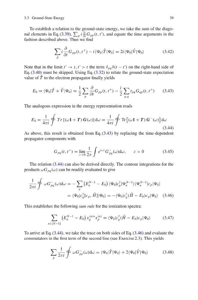
To establish a relation to the ground-state energy, we take the sum of the diagonal elements in Eq. (3.39),
p i
∂
∂t
G pp (t, t
), and equate the time arguments in the
fashion described above. Thus we find
p
i
∂
∂t
G pp (t, t
+
) − i 0 | ˆ
T | 0 = 2i 0 | ˆ
V | 0
(3.42)
Note that in the limit t
→ t, t
> t the term δ pq δ(t − t
) on the right-hand side of
Eq. (3.40) must be skipped. Using Eq. (3.32) to relate the ground-state expectation
value of ˆ
T to the electron propagator finally yields
E 0 = = 0 | ˆ
T + ˆ
V | 0 =
1
2
p
∂
∂t
G pp (t, t
+
) −
i
2
p,q
t pq G qp (t, t
+
)
(3.43)
The analogous expression in the energy representation reads
E 0 =
1
4πi
2 T r [(ω1 + T ) G(ω)] dω =
1
4πi
2 Tr
(ω1 + T ) G
−
(ω)
dω
(3.44)
As above, this result is obtained from Eq. (3.43) by replacing the time-dependent
propagator components with
G pq (t, t
+
) = lim
ε→0
1
2π
e
iωε G
−
pq (ω)dω,
ε > 0
(3.45)
The relation (3.44) can also be derived directly. The contour integrations for the
products ωG pq (ω) can be readily evaluated to give
1
2πi
2 ωG
−
pq (ω)dω = −
n
E
N −1
n
− E 0
0 |c
†
q |
N −1
n
N −1
n
|c p | 0
= = 0 |c
†
q [c p , ˆ
H ]| 0 = −− 0 |c
†
q ( ˆ
H − E 0 )c p | 0 (3.46)
This establishes the following sum rule for the ionization spectra:
n∈{N −1}
E
N −1
n
− E 0
x
(n)∗
q
x
(n)
p = = 0 |c
†
q ( ˆ
H − E 0 )c p | 0
(3.47)
To arrive at Eq. (3.44), we take the trace on both sides of Eq. (3.46) and evaluate the
commutators in the first term of the second line (see Exercise 2.3). This yields
p
1
2πi
2 ωG
−
pp (ω)dω = = 0 | ˆ
T | 0 + 2 0 | ˆ
V | 0
(3.48)
39
To establish a relation to the ground-state energy, we take the sum of the diagonal elements in Eq. (3.39),
p i
∂
∂t
G pp (t, t
), and equate the time arguments in the
fashion described above. Thus we find
p
i
∂
∂t
G pp (t, t
+
) − i 0 | ˆ
T | 0 = 2i 0 | ˆ
V | 0
(3.42)
Note that in the limit t
→ t, t
> t the term δ pq δ(t − t
) on the right-hand side of
Eq. (3.40) must be skipped. Using Eq. (3.32) to relate the ground-state expectation
value of ˆ
T to the electron propagator finally yields
E 0 = = 0 | ˆ
T + ˆ
V | 0 =
1
2
p
∂
∂t
G pp (t, t
+
) −
i
2
p,q
t pq G qp (t, t
+
)
(3.43)
The analogous expression in the energy representation reads
E 0 =
1
4πi
2 T r [(ω1 + T ) G(ω)] dω =
1
4πi
2 Tr
(ω1 + T ) G
−
(ω)
dω
(3.44)
As above, this result is obtained from Eq. (3.43) by replacing the time-dependent
propagator components with
G pq (t, t
+
) = lim
ε→0
1
2π
e
iωε G
−
pq (ω)dω,
ε > 0
(3.45)
The relation (3.44) can also be derived directly. The contour integrations for the
products ωG pq (ω) can be readily evaluated to give
1
2πi
2 ωG
−
pq (ω)dω = −
n
E
N −1
n
− E 0
0 |c
†
q |
N −1
n
N −1
n
|c p | 0
= = 0 |c
†
q [c p , ˆ
H ]| 0 = −− 0 |c
†
q ( ˆ
H − E 0 )c p | 0 (3.46)
This establishes the following sum rule for the ionization spectra:
n∈{N −1}
E
N −1
n
− E 0
x
(n)∗
q
x
(n)
p = = 0 |c
†
q ( ˆ
H − E 0 )c p | 0
(3.47)
To arrive at Eq. (3.44), we take the trace on both sides of Eq. (3.46) and evaluate the
commutators in the first term of the second line (see Exercise 2.3). This yields
p
1
2πi
2 ωG
−
pp (ω)dω = = 0 | ˆ
T | 0 + 2 0 | ˆ
V | 0
(3.48)